GPUs Learn to Think

It is September 2012. A convolutional network trained by two graduate students on a pair of gaming graphics cards wins the ImageNet competition by a margin the field has not seen before, and the chips that render video games become, almost overnight, the substrate of machine learning. The path there ran through a card that was never meant to do this — a graphics processor that a programming model called CUDA had quietly turned into a general-purpose parallel computer five years earlier.

Where We Were

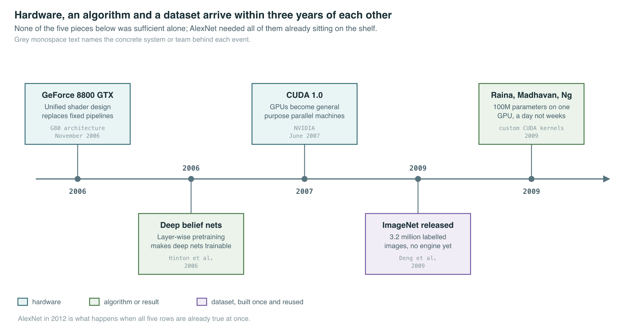
By the mid-2000s, neural networks had the ingredients to work and almost nowhere to run. Chapter 1 covers the thesis in full: deep belief nets could now be pretrained layer by layer, and a large labeled image dataset — ImageNet, released in 2009 — was on the way. What was missing was throughput. CPUs of the era added performance mostly by raising clock speed and adding a few cores, and training a network with millions of parameters on millions of examples meant looping over billions of multiply-accumulate operations, one core at a time, for weeks.

Graphics cards had spent the previous decade solving an unrelated problem — shading millions of independent pixels every frame — with an architecture that happened to be exactly what the neural-network problem needed. Rendering a frame means computing, for every pixel, a largely independent function of its position, its texture data, and a handful of lights; there is enormous work to do, but almost none of it depends on the pixel next to it. Chipmakers had already built hardware for exactly that shape of problem: hundreds of small, simple cores that all run the same instruction on different data at once, rather than a handful of large cores each doing something different. In November 2006, NVIDIA’s GeForce 8800 GTX introduced the G80 architecture with a unified, programmable shader design, replacing the older split of fixed-function vertex and pixel pipelines with a single pool of general-purpose cores that graphics workloads could be scheduled onto flexibly. In June 2007, NVIDIA released CUDA 1.0, a C-like programming model that let developers write general-purpose parallel programs for that hardware directly, without disguising ordinary computation as a graphics operation to smuggle it onto the chip. A GPU stopped being a device you could only reach through a graphics API and became a device you could program like any other processor, just one with a very different, and very useful, shape.

Part of why this mattered is that the alternative was running out of headroom. For decades, a slower processor could be made faster mainly by raising its clock speed, and each new generation of chips did that reliably. By the mid-2000s, that path was running into power and heat limits: pushing clock speed further cost disproportionately more energy per operation, so chipmakers redirected their transistor budgets toward adding more cores rather than making each core faster. A neural network training loop, expressed as a single sequential program, could not benefit from those extra cores at all — it needed to be rewritten as many small, independent pieces of work, which is exactly the shape a GPU’s hundreds of simple cores expect.

The gap between “GPUs can now run arbitrary parallel code” and “GPUs can train the deep networks the field wants to train” still had to be closed by hand. Early GPU deep learning was DIY: researchers wrote their own CUDA kernels for the operations they needed, because no shared library existed yet to do it for them. Every lab that wanted GPU speed had to also become, temporarily, a GPU-kernel-writing shop.

The Breakthrough

The first demonstration that this mattered at scale came from Stanford. Raina, Madhavan, and Ng showed that deep belief networks and sparse coding models — the workhorses of 2009-era unsupervised learning — could be trained on a single NVIDIA GPU, using custom CUDA kernels for the core matrix operations (Raina, Madhavan, and Ng, 2009). Their headline result was scale, not just speed: models with up to 100 million free parameters that would previously have required weeks on a CPU cluster became trainable in about a day on one desktop GPU. The insight the paper stated explicitly, and that the rest of the chapter follows, was that these unsupervised learning algorithms map naturally onto the highly parallel structure of a GPU because the bulk of their work is dense linear algebra, repeated identically across many independent data points.

Three years later, that insight met a bigger dataset and a bigger network. Krizhevsky, Sutskever, and Hinton, at the University of Toronto, built a convolutional network, later known as AlexNet, with about 60 million parameters across eight learned layers: five convolutional layers and three fully connected layers (Krizhevsky, Sutskever, and Hinton, 2012). The network was too large to fit in the 3 GB of memory on a single NVIDIA GTX 580 — a consumer gaming GPU from NVIDIA’s GTX 500 series, the same line that launched at $499 in November 2010 with less memory — so the authors split it across two GPUs, with the two halves communicating directly over the cards’ peer link only at specific layers to limit synchronization overhead. Training ran for five to six days. There was no cuDNN yet; the convolution kernels were written by hand in CUDA, in a codebase Krizhevsky released as cuda-convnet.

In the ImageNet Large Scale Visual Recognition Challenge results announced in September 2012, AlexNet reached a top-5 error rate of 15.3%, against 26.2% for the second-place entry — a margin so large relative to the field’s usual year-over-year gains that it was read immediately as a discontinuity rather than an increment. Splitting the network across two GPUs was not merely a memory workaround: the authors reported that the cross-GPU version reduced top-1 and top-5 error by 1.7 and 1.2 percentage points respectively compared with a same-sized network trained on one GPU, because more GPUs meant a bigger network fit in the same wall-clock training budget.

The architecture itself made choices that only paid off because a GPU could execute them cheaply at scale: the network used rectified linear units rather than the tanh or sigmoid nonlinearities common at the time, because a rectified linear unit is a single comparison against zero and is faster to compute, in bulk, across millions of neurons per layer than a saturating function. It also relied on dropout — randomly zeroing a fraction of neuron activations during training — to control overfitting in a network large enough that only GPU-scale compute made training it feasible at all. None of these choices were new in isolation; what was new was a single system where all of them ran fast enough, on affordable hardware, to be combined at this scale and evaluated on this benchmark.

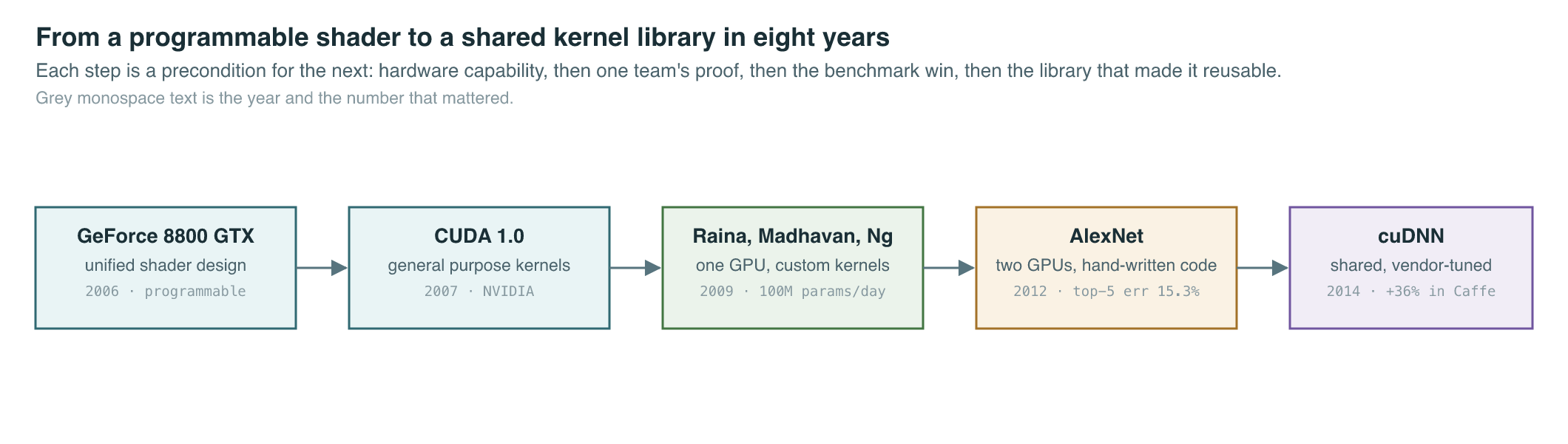
The gap AlexNet exposed was that every lab writing GPU deep learning code was re-deriving the same low-level kernels — convolution, pooling, activation functions — by hand, with no shared, professionally optimized implementation to build on. That duplication was expensive in a specific way: a convolution kernel tuned for one GPU generation’s memory layout and register file could lose much of its advantage on the next generation, so each hardware refresh forced every lab that cared about speed to re-tune its kernels from scratch, work with no scientific payoff of its own. NVIDIA closed that gap with cuDNN, a library of GPU-accelerated primitives for deep learning, modeled deliberately on BLAS, the decades-old standard for GPU and CPU linear algebra that numerical software had relied on for exactly this reason since the 1970s (Chetlur et al., 2014). Rather than every framework author hand-tuning convolution loops for each new GPU generation, cuDNN gave them one library to call, written and maintained by the hardware vendor and tuned for its own silicon — the tuning work amortized once, by the party with the deepest knowledge of the chip, instead of repeated once per framework per GPU generation. Integrating cuDNN into the Caffe framework improved performance by 36% on a standard model while also reducing memory consumption — a result achieved with no change to the network architecture, purely from a better-optimized kernel underneath it. cuDNN turned GPU deep learning from a craft, where results depended on how good your hand-written kernels were, into an engineering discipline built on a shared, swappable layer.

The Mathematics

The reason both papers in this chapter reach for a GPU rather than a faster CPU is that the dominant operation inside a neural network — and, after the “flatten the image patches” transform known as im2col, inside a convolutional layer specifically — is a large dense matrix multiplication. For two matrices $A$ (shape $m \times k$) and $B$ (shape $k \times n$), computing the product costs:

$$\mathrm{FLOPs}(A, B) = 2mnk$$

Symbol	Meaning
$A$	left matrix, shape $m \times k$ — unrolled input patches
$B$	right matrix, shape $k \times n$ — filter weights
$m, n$	output matrix dimensions
$k$	the shared inner dimension summed over in each dot product
$\mathrm{FLOPs}$	total multiply-add operations, counted as 2 per term

This is why the two papers in this chapter, from very different problem domains, converge on the same conclusion: a workload dominated by large matrix multiplications is a workload a GPU is unusually well suited to run, because the operation decomposes into millions of independent pieces of arithmetic with no data dependency between them. A GPU’s execution model reflects this directly — its cores are grouped so that a batch of them executes the identical instruction on different data in lockstep, an arrangement usually called SIMT, for single instruction, multiple threads. That arrangement is a poor fit for code full of data-dependent branching, but it is close to a perfect fit for a loop that performs the same multiply-and-accumulate on a different slice of a matrix on every iteration — which is precisely what a convolution, unrolled into a matrix multiply, is.

That suitability has a general name: Amdahl’s Law, formalized by Gene Amdahl in 1967 to describe the limits of parallel processing regardless of processor count. If a fraction $f$ of a program’s total work can be split across independent parallel processors and the remaining fraction $1-f$ must run sequentially, then running the parallel portion on $P$ processors instead of one gives a speedup of:

$$S(P) = \frac{1}{(1 - f) + \dfrac{f}{P}}$$

What It Enabled

	Before, CPU-only deep learning	After, GPU-accelerated deep learning
Representative hardware	Multi-core CPU clusters	1–2 consumer gaming GPUs (GTX 280, GTX 580)
Reported training time	Weeks, for large unsupervised models (Raina et al., 2009 baseline)	About a day for 100M-parameter models (Raina et al., 2009); five to six days for the 60M-parameter AlexNet (2012)
Convolution kernel source	None shared — hand-written per project	Hand-written per project (2012) → shared vendor library, cuDNN (2014)
ImageNet top-5 error (2012 competition)	26.2% (best non-AlexNet entry)	15.3% (AlexNet)
Framework kernel maintenance	Each research group maintained its own	One vendor library, patched once, used everywhere

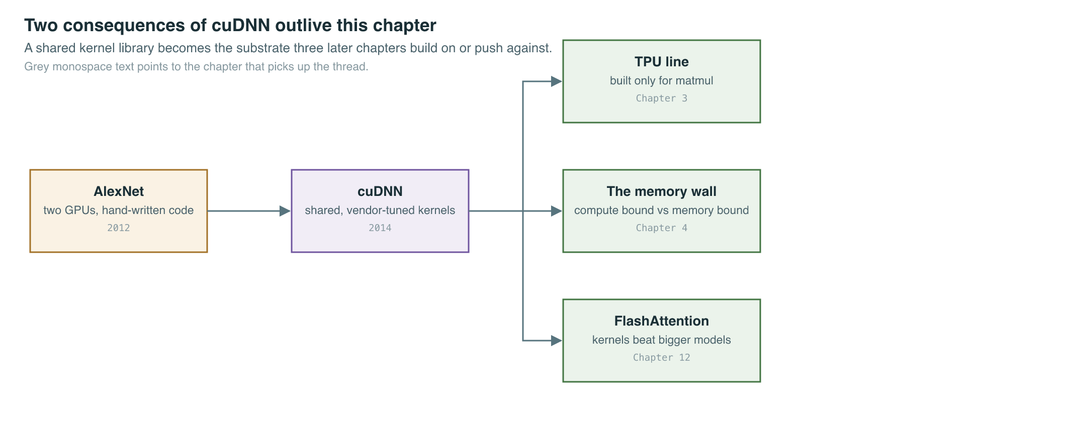
The two-part shift — GPUs first as a raw speed multiplier, then cuDNN as a shared, professionally optimized layer underneath every framework — set the terms that the rest of this book’s Part I builds on. Deep learning frameworks that emerged over the following years, rather than each maintaining their own convolution and pooling kernels, increasingly called into cuDNN underneath a higher-level Python or Lua interface, which meant a framework’s speed on NVIDIA hardware was, to a first approximation, cuDNN’s speed. That separation of “framework on top, vendor kernel library underneath” is still the shape of the deep learning software stack: PyTorch and JAX both call into cuDNN or its descendants for the same operations this chapter describes.

Once one accelerator vendor’s programmable hardware had proven itself on the field’s flagship benchmark, other accelerator designs entered the race, most consequentially Google’s TPU line, covered in Chapter 3, which asked whether a chip built only for the matrix-multiply pattern this chapter’s mathematics describes could out-specialize a general-purpose GPU. Once GPU memory, rather than compute, became the binding constraint on model size — the very problem that forced AlexNet onto two cards — the field needed a systematic account of when a workload is compute-bound versus memory-bound, which is the subject of Chapter 4. Splitting a single model across multiple GPUs, done here by hand for one network, became its own discipline as models grew past what any GPU’s memory could hold, covered in Chapter 9. And once a shared kernel library existed at all, the idea that the fastest path to new capability might run through better kernels, not just bigger models, became a recurring pattern — one that resurfaces directly with FlashAttention a decade later, in Chapter 12.

The fit this chapter documents between matrix-multiply-heavy architectures and GPU parallelism is also what the Transformer would exploit far more fully a few years later: an architecture built almost entirely out of the same dense matrix multiplications this chapter’s math describes, at a scale CUDA and cuDNN made merely conceivable rather than yet practical (language models, Chapter 5).

Key Papers

Paper	Authors	Year	Link	Why it matters
Large-scale Deep Unsupervised Learning Using Graphics Processors	Raina, Madhavan, and Ng	2009	doi:10.1145/1553374.1553486	First demonstration that a single GPU, programmed via CUDA, could train deep unsupervised models with up to 100 million parameters in about a day
ImageNet Classification with Deep Convolutional Neural Networks	Krizhevsky, Sutskever, and Hinton	2012	doi:10.1145/3065386	AlexNet’s ILSVRC-2012 win on two consumer GPUs made GPU-trained deep learning the field’s default, virtually overnight
cuDNN: Efficient Primitives for Deep Learning	Chetlur et al.	2014	arXiv:1410.0759	Replaced hand-written per-project convolution kernels with a shared, vendor-optimized library, the model every later kernel library follows

PM Lens