The Memory Wall

It is April 2009. GPUs have spent barely two years as general-purpose processors, and the deep-learning boom this book’s early chapters describe has not yet started. In Communications of the ACM, three researchers from the University of California, Berkeley and Lawrence Berkeley National Laboratory publish a one-page chart built to answer a narrower question: for a given piece of code on a given chip, is the ceiling on speed set by how fast the chip computes, or by how fast it can be handed data? Fifteen years later, that same chart is the first thing a systems engineer reaches for to explain why a large language model serves tokens at the speed it does, and no faster.

Where We Were

The gap the chart answers had a name for over a decade before it had a widely used chart. In 1995, Wulf and McKee observed that processor speed had been improving, year over year, far faster than DRAM access latency, and warned that if the trend continued, most programs would stop being limited by how fast a processor could compute and start being limited by how fast it could be handed data from main memory — a condition they named the memory wall (Wulf and McKee, 1995). Their argument was architecture-agnostic: it applies to any processor whose compute throughput grows faster than the bandwidth and latency of the memory feeding it, which by the mid-1990s was already every processor on the market.

GPUs arrived at the same tension from a different direction. Chapter 2 covers how CUDA, released in 2007, turned graphics chips into general-purpose parallel computers, and how Raina, Madhavan, and Ng trained deep unsupervised models on a single GPU two years later. Both of those results were framed, correctly, as compute stories: more parallel arithmetic units meant more FLOPs per second, and more FLOPs per second meant faster training. But a chip’s peak FLOPs figure, printed on a vendor’s spec sheet, is a ceiling that a given piece of code may or may not come anywhere near. AlexNet’s authors, splitting their network across two GPUs in 2012, were already running into the other half of the story: a workload can be limited by how much data has to move in and out of the chip’s memory, not by how many arithmetic units sit idle waiting for that data to arrive.

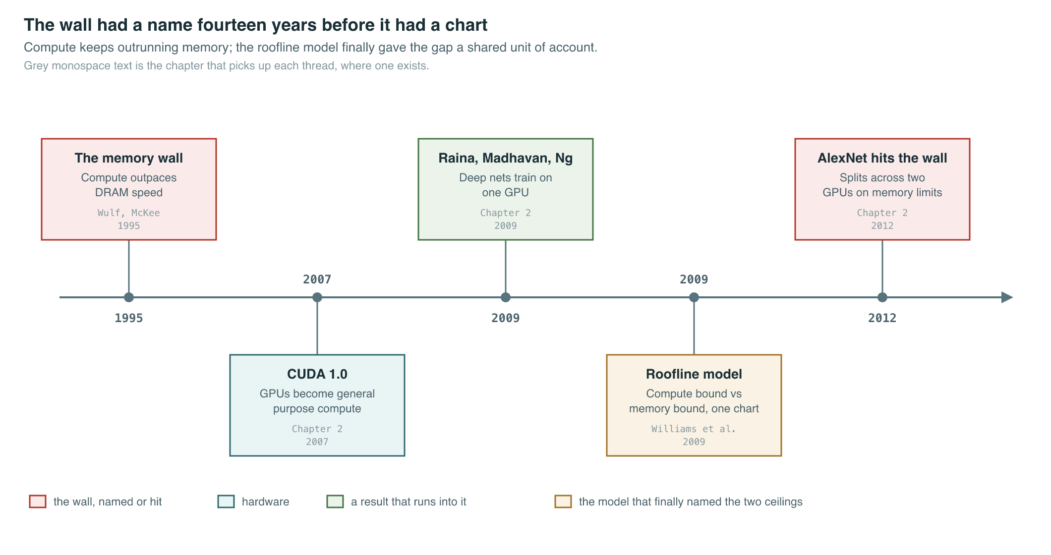
The gap had a name fourteen years before it had a chart; the roofline model is what finally let engineers say which ceiling a given kernel was hitting. PNG ↓

Before 2009, there was no shared, quantitative vocabulary for diagnosing which side of that divide a given kernel fell on. A benchmark either ran fast or it didn’t; a vendor’s marketing FLOPs number was either close to what you measured or it wasn’t, and nobody had a simple way to say, in advance, which outcome to expect for a specific piece of code. Two chips with identical peak FLOPs could deliver wildly different real-world performance on the same program if their memory systems differed, and a program that hit 5% of a chip’s peak FLOPs might be badly written, or it might already be running exactly as fast as the laws of arithmetic and the chip’s memory bus allow. Without a model that separated those two explanations, performance engineering was mostly guesswork dressed up as intuition.

The Breakthrough

Williams, Waterman, and Patterson answered the question with a single log-log plot (Williams et al., 2009). On the horizontal axis sits a property of the code being run, called operational intensity: how many floating-point operations the program performs for every byte it moves between main memory and the processor. On the vertical axis sits attainable performance, in FLOPs per second. Two lines bound every possible point on that plot. A horizontal line marks the chip’s peak compute throughput — no program can run faster than the chip’s arithmetic units allow, no matter how efficiently it uses memory. A diagonal line, rising at a slope set by the chip’s peak memory bandwidth, marks the fastest a program can run if it is limited purely by how fast data arrives — no program can outrun the rate at which its inputs and outputs cross the memory bus. The two lines meet at a single point, the ridge point, and a piece of code’s operational intensity determines which line applies to it: to the left of the ridge point, a kernel is memory-bound and the diagonal bandwidth line is the ceiling; to the right, it is compute-bound and the flat FLOPs line is the ceiling. The resulting shape — flat roof, sloped roof, ridge where they meet — is the “roofline” the paper is named for.

The model’s origin was multicore CPU performance analysis: the paper measured kernels like sparse matrix-vector multiply, structured-grid stencils, and dense matrix multiply on early-2000s multicore chips, and used the roofline to show which kernels had headroom left to optimize and which had already hit a hard architectural ceiling. Williams, Waterman, and Patterson were explicit that the model is a bound, not a prediction: it tells you the fastest a kernel with a given operational intensity could possibly run on a given chip, and whether a measured result is close to that ceiling or far below it — which is a different, more actionable question than “is this fast.” A kernel sitting right on its roofline cannot be sped up by better code; it can only be sped up by increasing its operational intensity or by using a chip with a higher roof. A kernel sitting well below its roofline has a software problem, not a hardware one.

Operational intensity is a property of an algorithm’s data-reuse pattern, not of the chip it happens to run on, and that portability is what let the same chart travel from CPUs to GPUs to the accelerators this book’s Part I covers. The chip side of the ratio — peak FLOPs against peak bandwidth — is set by where the chip spends its transistor and power budget, and that split is itself shaped by the physical path data has to travel: from the processor’s registers, to its on-chip SRAM, out to off-chip DRAM, and, for multi-chip training runs, across an interconnect and possibly a network link, with bandwidth dropping by roughly an order of magnitude at each hop outward.

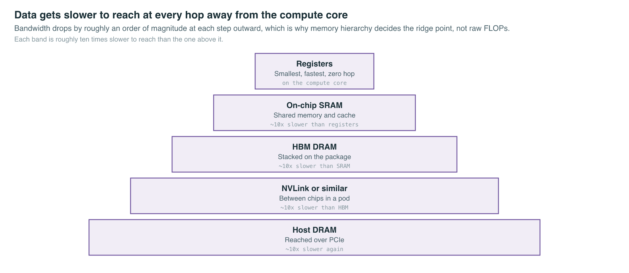
Bandwidth drops by about an order of magnitude at every hop away from the compute core, which is why memory hierarchy, not raw FLOPs, decides where the ridge point sits. PNG ↓

The specific technology that widened the diagonal roofline for accelerators was High Bandwidth Memory, or HBM: DRAM dies stacked vertically and placed a few millimeters from the compute die on the same package, connected by thousands of short, wide wires instead of the long, narrow traces that off-package GDDR memory needs. Stacking and shortening the path raises achievable bandwidth substantially over off-package memory at a given power budget, which is why every data-center GPU and TPU generation this book covers is built around HBM rather than the graphics-card memory of a decade earlier. It does not remove the wall; it moves the ridge point, and, as the numbers below show, compute throughput has kept moving it back.

The Mathematics

Operational intensity is the ratio at the center of the whole model. For a piece of code that performs $W$ total floating-point operations while moving $Q$ total bytes between DRAM and the processor over its execution:

I = \frac{W}{Q}

Attainable performance is then bounded by whichever ceiling operational intensity puts the code under:

P = \min\!\big(P_{\text{peak}},\; I \times BW_{\text{peak}}\big)

Symbol	Meaning
$P$	Attainable performance, in floating-point operations per second
$P_{\text{peak}}$	The chip’s peak compute throughput, the flat roof
$I$	Operational intensity of the code, in FLOPs per byte
$BW_{\text{peak}}$	The chip’s peak memory bandwidth, in bytes per second, setting the slope of the diagonal roof

The point where the two ceilings meet — the ridge point — is a property of the chip alone, independent of any particular piece of code:

I_{\text{ridge}} = \frac{P_{\text{peak}}}{BW_{\text{peak}}}

Dividing the chip’s peak compute throughput by its peak bandwidth gives the operational intensity at which a kernel exactly saturates both the arithmetic units and the memory bus at once — the exact spot where the flat roof and the sloped roof cross. What it buys you: any code with operational intensity below $I_{\text{ridge}}$ for a given chip is memory-bound on that chip and cannot be sped up by writing tighter arithmetic; any code above $I_{\text{ridge}}$ is compute-bound and cannot be sped up by moving data more cleverly. $I_{\text{ridge}}$ is sometimes called the chip’s machine balance, and as the next section shows, it has been rising for two decades — meaning the bar an algorithm must clear to stay compute-bound keeps moving up, even as the algorithm itself stays the same.

Two families of operation illustrate the ridge point in practice. A large dense matrix multiplication — the operation Chapter 2 shows dominating both AlexNet’s convolutions and, later, every transformer layer — reuses each loaded value many times across a big output tile before it is evicted from on-chip storage, so its operational intensity grows with the tile size and, at large enough scale, comfortably clears most chips’ ridge points: dense GEMM is the canonical compute-bound kernel. An elementwise operation — adding a residual, applying an activation function, or normalizing a vector — performs on the order of one arithmetic operation per value it reads and writes, so its operational intensity is small and roughly fixed regardless of problem size: elementwise kernels are memory-bound on essentially every chip built since the mid-1990s wall Wulf and McKee described. Standard self-attention sits closer to the elementwise end than the GEMM end for a structural reason that has nothing to do with how carefully it is coded: computing attention scores for every pair of tokens produces an intermediate matrix whose size grows with the square of the sequence length, and if that matrix has to be written out to and read back from DRAM in full, the memory traffic grows with it — which is exactly the constraint that motivates the IO-aware kernel design of FlashAttention, covered in full in Chapter 12 (Dao et al., 2022).

What It Enabled

The roofline model gave the field a shared unit of account: instead of arguing about whether a kernel was “fast,” engineers could ask where it sat relative to its chip’s ridge point, and whether the fix was an algorithm change or a hardware upgrade. Tracking how that ridge point has moved across accelerator generations makes the trend concrete.

Accelerator, launch	Peak Tensor Core throughput	HBM bandwidth per chip	Machine balance, FLOP per byte
V100, Volta, 2017	125 TFLOP/s FP16, dense	900 GB/s, HBM2	≈ 139
A100, Ampere, May 2020	312 TFLOP/s FP16, dense	2.04 TB/s, HBM2e	≈ 153
H100, Hopper, announced March 2022	≈ 990 TFLOP/s FP16, dense	3.35 TB/s, HBM3	≈ 295
B200, Blackwell, announced March 2024	≈ 9 PFLOP/s FP8, sparse	≈ 8 TB/s, HBM3e	≈ 1,125

The rows are not perfectly apples-to-apples — the last row reports a lower-precision, sparsity-assisted figure because that is the format NVIDIA’s own datasheet leads with for Blackwell, reflecting the industry’s own drift toward narrower number formats as a second lever against the wall, covered in Chapter 7 — but even with that caveat, the pattern is unmistakable: machine balance has risen roughly eightfold in seven years. HBM bandwidth has grown substantially at every generation, but peak compute throughput has grown faster still, which means the bar an algorithm must clear to stay compute-bound keeps climbing, even for algorithms — like attention — whose own operational intensity is fixed by their structure and does not automatically rise with the hardware.

That widening gap, more than any single paper, is the reason so much of this book’s remaining chapters exist. If compute were the only scarce resource, training and serving large models would be almost entirely a story about buying more FLOPs. Instead, because bandwidth has consistently lagged compute, a large share of systems engineering for deep learning is about reducing bytes moved rather than operations performed: sharding optimizer state and gradients so less of each fits in memory at once (Chapter 10), using narrower numeric formats so the same values cost fewer bytes to move (Chapter 7), compressing trained weights after the fact so inference reads fewer bytes per token (Chapter 15), routing each token through only a fraction of a model’s parameters so fewer weights need to be touched at all (Chapter 13), and, at serving time, managing a growing key-value cache so that generating each new token moves as few bytes as possible (Chapter 17). FlashAttention is the sharpest single example: it does not reduce the number of floating-point operations attention performs, and in fact performs some redundant recomputation — it reduces attention’s memory traffic, moving an algorithm that was memory-bound closer to the chip’s compute roof by changing $Q$ , not $W$ .

Naming the two ceilings turns into six different strategies for moving fewer bytes rather than performing fewer operations. PNG ↓

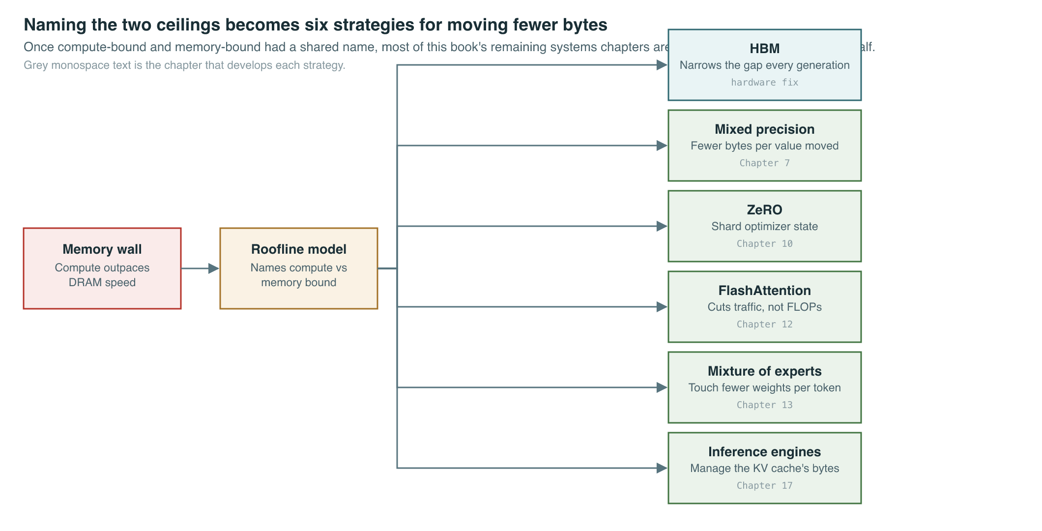
The same lens applies just as directly to serving a trained model as to training one, and for a similar reason: generating one token at a time from a large language model reads the full set of weights, and a growing key-value cache, from HBM for a comparatively tiny amount of arithmetic per token — a textbook memory-bound workload, sitting well to the left of the ridge point in the table above regardless of how fast the chip’s arithmetic units are. That is why buying a chip with more peak FLOPs does not proportionally speed up single-request LLM inference, and why the industry’s actual inference-cost roadmap runs through bandwidth-aware serving techniques rather than raw compute — the subject Chapter 17 covers in depth.

Key Papers

Paper	Authors	Year	Link	Why it matters
Hitting the Memory Wall: Implications of the Obvious	Wulf & McKee	1995	doi:10.1145/216585.216588	Named the structural gap between processor and memory speed that every later chapter in this book is, in some form, still responding to
Roofline: An Insightful Visual Performance Model for Multicore Architectures	Williams et al.	2009	doi:10.1145/1498765.1498785	Gave the field a single chart and formula for classifying any kernel as compute-bound or memory-bound on any chip
FlashAttention: Fast and Memory-Efficient Exact Attention with IO-Awareness	Dao et al.	2022	arXiv:2205.14135	The clearest later example of the roofline logic applied deliberately: reduce memory traffic, not FLOPs, to move a memory-bound kernel toward its compute roof — covered in full in Chapter 12

PM Lens

Every vendor pitch I get for a new GPU or inference stack leads with a peak FLOPs number, and it is almost never the number that predicts what I actually pay per token. A recent on-demand price for an 8-H100 cloud instance has hovered around $55 an hour — call it $7 per GPU-hour — and the honest question when I am scoping an inference workload is not “how many FLOPs does this chip have,” it is “how much of my workload is memory-bound, and does this chip’s bandwidth, not its FLOPs, match that.” Single-request chat latency, small-batch fine-tuning jobs, and anything dominated by loading weights or a KV cache are memory-bound by this chapter’s own definition, so a chip with 3x the FLOPs and the same bandwidth buys almost nothing for them. What does move the needle — quantizing weights, batching more requests together, picking a serving engine that manages the KV cache well — all reduce bytes moved, not operations performed. When a vendor’s benchmark slide shows a huge FLOPs advantage but a modest real-world speedup, this chapter is usually why.

Search