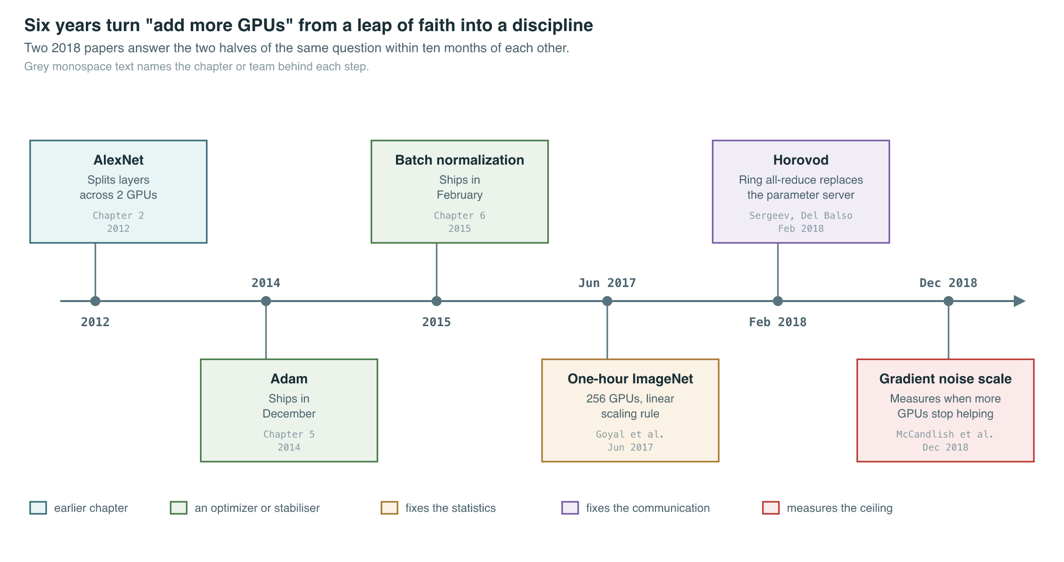
Data Parallelism and Large Batches

It is June 2017. ResNet-50 (owned by chapter 1) already trains on a single machine in a few days, but a few days per experiment means a few experiments per month, and every lab racing toward larger models wants more shots on goal. A Facebook team publishes a recipe for training the same network on 256 GPUs in one hour without losing accuracy, and a year and a half later an open-source library and a diagnostic statistic turn that recipe into a repeatable engineering discipline rather than a one-off stunt.

Where We Were

Splitting a single training run across more than one accelerator was not new by 2017. AlexNet (owned by chapter 2) had already split its layers across two GPUs in 2012 out of memory necessity, and by the mid-2010s it was routine to train on a handful of GPUs inside one server, connected by fast local interconnects. What was missing was a practical way to add the tenth GPU, or the hundredth — machines in different racks, connected by ordinary datacenter networking, coordinating on a single model.

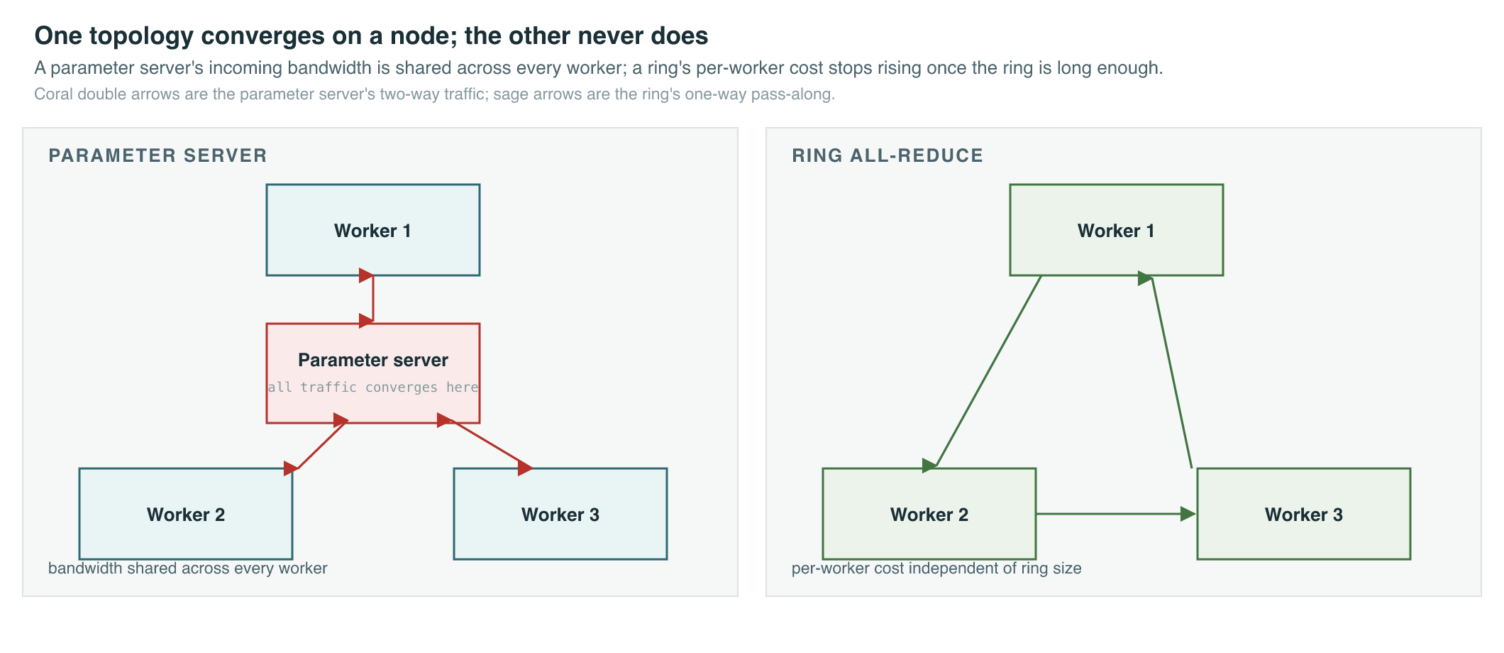
The obstacle was communication, not compute. Every accelerator added to a training run also added an obligation: after each accelerator computed its slice of the gradient, all the slices had to be combined and every accelerator had to end the step with the same updated weights, or the model would drift into inconsistent replicas. The dominant pattern for this, inherited from earlier large-scale machine learning systems, was the parameter server: one or a few dedicated nodes that received gradients from every worker, summed them, and broadcast the update back out. As the number of workers grew, so did the traffic converging on those few nodes, and the server’s bandwidth — not the accelerators’ compute — became the limiting resource. Doubling the worker count did not halve the wall-clock time; it moved the bottleneck instead.

There was a second, subtler obstacle sitting underneath the first. Even with unlimited bandwidth, nobody had a principled rule for how to adjust the optimizer when the batch size grew by 10× or 100×. The optimizers in question were themselves recent: Adam (owned by chapter 5) had shipped in December 2014, and batch normalization (owned by chapter 6) in February 2015, both tuned and validated at the batch sizes of the day — typically 256 or fewer images. Simply feeding an optimizer a much larger batch without adjusting anything else tended to produce a network that trained fast in wall-clock terms but generalized worse, and nobody could say in advance where that trade-off would bite.

Six years turn distributed training from ad hoc GPU-splitting into two measured disciplines: fixing the statistics and fixing the communication. PNG ↓

The Breakthrough

Act one: the linear scaling rule. “Accurate, Large Minibatch SGD: Training ImageNet in 1 Hour” (Goyal et al., 2017), submitted by a Facebook AI Research team in June 2017, attacked the optimizer half of the problem directly. The paper’s rule is stated in one sentence: “when the minibatch size is multiplied by k, multiply the learning rate by k,” holding every other hyperparameter — weight decay included — fixed. It is a hyperparameter-free prescription: no new tuning run is needed to find the right learning rate at a new batch size, because the rule derives it from the old one.

The rule alone was not sufficient. Applied naively from the first step of training, a learning rate scaled up 32× (to match a minibatch scaled from 256 to 8,192 images) was large enough to destabilize the network before it had learned anything. The paper’s second contribution was a warmup schedule: rather than jumping to the target learning rate immediately, gradually increase it from a small value over the first five epochs. A constant low-then-high warmup helped somewhat; a gradual, linear ramp helped more, and was the version the paper adopted. With gradual warmup and the linear scaling rule, a minibatch of 8,192 images spread across 256 GPUs matched the accuracy of the small-minibatch baseline — 23.60% top-1 error at minibatch 256 versus 23.74% at minibatch 8,192, a gap smaller than the run-to-run noise — and did so while training ResNet-50 on ImageNet in one hour instead of days. The paper also reported the edges of the recipe: results degraded past roughly 16,000 images per minibatch, and training diverged entirely beyond 64,000.

Act two: the communication layer. Getting 256 GPUs to agree on a gradient in the first place was the second half of the problem, and it was solved by treating the parameter server itself as the thing to remove. “Horovod: fast and easy distributed deep learning in TensorFlow” (Sergeev and Del Balso, 2018), submitted by a team at Uber in February 2018, replaced the server-centric topology with ring all-reduce: workers are arranged in a logical ring, and gradients are summed by passing partial sums around the ring rather than converging on a central node. Sergeev and Del Balso cite the earlier analysis by Patarasuk and Yuan showing this algorithm is bandwidth-optimal — for a large enough message, every worker’s incoming and outgoing traffic is the same regardless of how many workers are in the ring, so adding workers stops adding a communication tax. Horovod packaged this as a library that needed, in the authors’ words, only “a few lines of modification to user code,” turning a systems-engineering problem into an import statement.

The measured effect was the point. Standard distributed TensorFlow of the period, using the parameter-server pattern, delivered roughly 50% scaling efficiency at 128 GPUs — half the compute added was lost to communication. Horovod’s ring all-reduce reached 88% scaling efficiency on Inception V3 and ResNet-101 over a standard 25GbE TCP network at the same GPU counts, and over 90% on RDMA networking. Together, the linear scaling rule and ring all-reduce answered the two halves of the same question: how to keep the statistics of training correct as the batch grows, and how to keep the communication cheap as the worker count grows.

A parameter server's incoming bandwidth is shared across every worker; a ring's per-worker cost stops rising once the ring is long enough to hide the latency term. PNG ↓

The Mathematics

The linear scaling rule follows from comparing two ways of consuming the same data. Take $k$ small steps of batch size $n$ each, or one large step of batch size $kn$ :

\begin{aligned} w_{t+k} &= w_t - \eta \, \frac{1}{n} \sum_{j<k} \sum_{x \in B_j} \nabla_w \, l(x, w_{t+j}) \\ \hat{w}_{t+1} &= w_t - \hat{\eta} \, \frac{1}{kn} \sum_{j<k} \sum_{x \in B_j} \nabla_w \, l(x, w_t) \end{aligned}

Symbol	Meaning
$w_t$	Model weights at step $t$
$\eta$	Baseline learning rate, small-batch
$\hat{\eta}$	Scaled learning rate, large-batch
$n$	Small-batch size
$k$	Number of small steps folded into one big step
$B_j$	The $j$ -th minibatch of size $n$
$l(x, w)$	Per-example loss

Ring all-reduce’s communication cost, the property Horovod exploited, has a standard closed form as a function of worker count:

T_{\mathrm{ring}}(p) = 2(p-1)\,\alpha + 2\,\frac{p-1}{p}\,\frac{M}{\beta}

$T_{\mathrm{ring}}$ is the time to average gradients across $p$ workers, each holding a gradient buffer of $M$ bytes, over a network with per-message latency $\alpha$ and bandwidth $\beta$ . The first term grows with $p$ — more workers means more hops around the ring — but for realistically large gradient buffers it is the second term that dominates, and $(p-1)/p$ approaches 1 as $p$ grows. That means the bandwidth term converges to $2M/\beta$ , a constant independent of how many workers are in the ring. This is the mathematical content of “bandwidth-optimal”: unlike a parameter server, whose incoming bandwidth is shared across all workers and therefore degrades as $p$ grows, a ring’s per-worker communication cost stops rising once the ring is long enough to hide the latency term.

Symbol	Meaning
$T_{\mathrm{ring}}$	Time to complete one all-reduce across the ring
$p$	Number of workers in the ring
$\alpha$	Fixed latency per network message
$M$	Size of the gradient buffer being reduced, in bytes
$\beta$	Achievable network bandwidth

Neither result says how large a batch should be — only how to train correctly at a given size and how to communicate cheaply while doing it. “An Empirical Model of Large-Batch Training” (McCandlish et al., 2018), submitted by OpenAI in December 2018, supplied the missing instrument: a single statistic, measurable during training, that predicts the batch size beyond which adding more data per step stops helping.

\mathcal{B}_{\mathrm{simple}} = \frac{\operatorname{tr}\big(\Sigma(\theta)\big)}{\lVert G(\theta) \rVert^2}, \qquad \Sigma(\theta) = \mathbb{E}_{x \sim \rho}\!\left[\nabla_\theta L_x(\theta)\,\nabla_\theta L_x(\theta)^{\top}\right] - G(\theta)G(\theta)^{\top}

$G(\theta)$ is the true gradient of the loss — the direction training would follow with infinite data per step. $\Sigma(\theta)$ is the covariance of the noisy per-example gradients $\nabla_\theta L_x(\theta)$ around that true direction: how much a single example’s gradient disagrees with the average. The noise scale $\mathcal{B}_{\mathrm{simple}}$ is the ratio of that disagreement (summed across all parameters via the trace, $\operatorname{tr}$ ) to the squared size of the true gradient — a signal-to-noise ratio for the gradient estimate, in units of examples. McCandlish et al. show this quantity predicts the critical batch size, $\mathcal{B}_{\mathrm{crit}}$ , the empirically observed point beyond which doubling the batch no longer roughly halves the number of steps needed: their central empirical claim is that $\mathcal{B}_{\mathrm{crit}} \approx \mathcal{B}_{\mathrm{noise}}$ , where $\mathcal{B}_{\mathrm{noise}}$ is this statistic averaged appropriately over training. Below the critical batch size, more data per step is nearly free — training is compute-efficient but you are not using all the parallel hardware you could; above it, more data per step buys progressively less — training is hardware-hungry but not compute-efficient. The noise scale turns “how many GPUs should this run use” from a guess into a measurement.

Symbol	Meaning
$G(\theta)$	True gradient of the loss at parameters $\theta$
$\Sigma(\theta)$	Covariance of per-example gradients around $G$
$L_x(\theta)$	Loss on a single example $x$
$\rho$	Data distribution examples are drawn from
$\operatorname{tr}(\cdot)$	Trace, summing variance across all parameter dimensions
$\mathcal{B}_{\mathrm{simple}}$	The measurable noise-scale statistic
$\mathcal{B}_{\mathrm{crit}}$	The empirical critical batch size it predicts

The paper also defines a Hessian-weighted version of the same quantity, $\mathcal{B}_{\mathrm{noise}} = \operatorname{tr}(H\Sigma) / (G^{\top} H G)$ , which reduces to the simple form above when the loss curvature $H$ is well approximated by a scaled identity matrix — a condition close enough to true in practice that the simple version is the one used for measurement.

Critically, McCandlish et al. found the noise scale is not a fixed property of a model or dataset: it grows as training proceeds and the network gets more accurate, and it is larger for harder tasks. Measured across domains, both the noise scale and the critical batch size it predicts span many orders of magnitude:

Task	Simple noise scale (examples)	Critical batch size (examples)
MNIST	50–900	20–200
SVHN	300–4,000	50–500
CIFAR-10	400–2,000	300–900
ImageNet	4,000–30,000	1,000–15,000
Billion Word (per token)	1,000–150,000	700–100,000
Atari (per frame)	100–20,000	100–8,000
Dota 1v1 (per frame)	100,000–300,000	50,000–3,000,000
Dota 5v5 (per frame)	up to 24,000,000	not measured

What It Enabled

The immediate effect was that “how many GPUs” stopped being an engineering leap of faith. Before Goyal et al. and Horovod, scaling a run past a handful of accelerators risked losing accuracy, communication overhead, or both, with no diagnostic to tell you which. After them, both failure modes had a fix — the linear scaling rule plus warmup for the first, ring all-reduce for the second — and the gradient noise scale gave a third answer: a number that told you when to stop adding workers before you started paying for hardware that made no difference.

Configuration	GPUs	Scaling efficiency	Source
Standard distributed TensorFlow, parameter server	128	~50%	Sergeev and Del Balso, 2018
Horovod, ring all-reduce, TCP 25GbE	128	88%	Sergeev and Del Balso, 2018
Horovod, ring all-reduce, RDMA	128	over 90%	Sergeev and Del Balso, 2018
Goyal et al. distributed SGD, linear scaling + warmup	8 to 256	~90%	Goyal et al., 2017

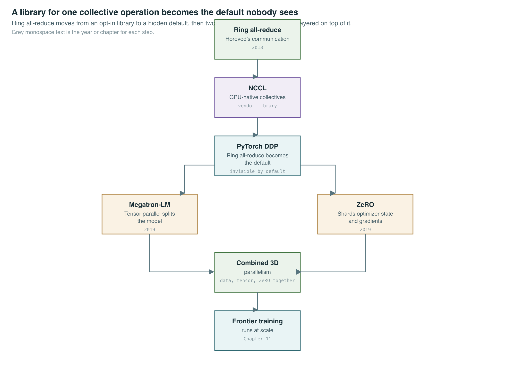
Ring all-reduce did not stay a Horovod-only technique. NVIDIA’s NCCL library implemented the same collective operation as a GPU-aware primitive, and PyTorch’s built-in DistributedDataParallel adopted ring all-reduce as its default gradient-synchronization strategy, making the pattern from this chapter the invisible default for essentially every multi-GPU training job that followed rather than an opt-in library. Data parallelism this chapter describes is only half of how a modern run is split, however — once a single model no longer fits on one accelerator regardless of batch size, the model itself has to be partitioned, which is the subject of chapter 9, splitting the model, and the memory accounting that decides when that partitioning becomes necessary is covered in chapter 10, ZeRO and the memory tricks. In practice, frontier training runs combine both — a topic taken up directly in chapter 11, training runs in practice.

The gradient noise scale’s longer legacy was conceptual as much as practical: it reframed batch size as something with a measurable ceiling rather than a hyperparameter to search over. That same instinct — that a resource has a knowable, fitted relationship to training outcomes rather than an empirically groped-for setting — is the premise the field generalized two years later into predicting loss itself from parameters, data, and compute, the subject of scaling laws. The connection is not incidental: the gradient noise scale is, in effect, a scaling law for the batch-size axis alone, published by three of the same authors — McCandlish, Kaplan, and Amodei — who wrote the language-model scaling laws paper thirteen months later. Both papers ask the same underlying question, “what is the exchange rate between more hardware and less wall-clock time,” and both answer it with a curve fitted to small, cheap experiments rather than a rule of thumb.

Ring all-reduce stops being an opt-in library and becomes the invisible default, while two more axes of splitting the model and its state get layered on top. PNG ↓

Large-batch training also intersected with the hardware roadmap. Bigger batches only pay off if there is enough accelerator memory and interconnect bandwidth to hold and synchronize them, which is why the memory wall and the pace of GPU generations described in the co-evolution thesis set a practical ceiling on how far the linear scaling rule can be pushed before communication or memory, not statistics, becomes the binding constraint again.

Key Papers

Paper	Authors	Year	Link	Why it matters
Accurate, Large Minibatch SGD: Training ImageNet in 1 Hour	Goyal et al.	2017	arXiv:1706.02677	Linear scaling rule plus warmup made large-batch training accuracy-preserving
Horovod: fast and easy distributed deep learning in TensorFlow	Sergeev and Del Balso	2018	arXiv:1802.05799	Ring all-reduce replaced parameter servers as the default communication pattern
An Empirical Model of Large-Batch Training	McCandlish et al.	2018	arXiv:1812.06162	Gradient noise scale predicts the batch size beyond which more workers stop helping

PM Lens

When a training-infra team tells me a run needs “more GPUs,” this chapter is the checklist I reach for before signing off on the spend. First: is the batch-size increase actually paired with the linear scaling rule and a warmup schedule, or is someone just cranking a knob and hoping accuracy holds? Second: is the cluster using ring all-reduce — the PyTorch and NCCL default today — or has someone reinvented a parameter-server bottleneck without realizing it? Third, and the one people skip: has anyone measured the gradient noise scale for this workload, or are we just adding workers until the cloud bill hurts? I have watched teams double a cluster and get a 10% speedup, not because the tooling was broken but because the run was already past its critical batch size — the extra GPUs were computing a gradient nobody needed more precision on. The 2017–2018 papers in this chapter did not just make big clusters usable; they gave everyone downstream a way to tell a good scale-up from an expensive one.

Search