Scaling Laws

It is January 2020. The transformer is two and a half years old, GPT-2 has shown that bigger generative models write better text, and every lab is asking the same question with no principled way to answer it: given a fixed budget of compute, how large should the model be, and how much data should it see? A ten-author paper from OpenAI turns that question from folklore into a fitted curve — and two years later, DeepMind shows the curve was fitted wrong.

Where We Were

By late 2019 the field had strong evidence that scale helped and almost no theory of how much. The Transformer (Vaswani et al., June 2017) had made training larger sequence models practical; GPT-2 (February 2019) had demonstrated that a generatively pretrained decoder improved broadly as it grew; T5 and BART (both October 2019) had pushed transfer learning across every text task. But sizing decisions were made by intuition and budget, not by prediction.

The practical questions compounded. Depth or width? More parameters or more data? Train to convergence or stop early? How large a batch? Work on large-batch training and gradient noise had begun to give partial answers for optimization, but nobody could say in advance what the loss of a ten-times-larger model would be, so every scale-up was a leap of faith justified after the fact.

The stakes were rising with the hardware. Training runs were moving from single machines to clusters, and a mistake in allocation — a model too large for its data, or data wasted on a model too small — burned weeks of accelerator time that could not be refunded. What the field needed was an instrument: something that let you measure small models cheaply and predict large ones before paying for them.

The Breakthrough

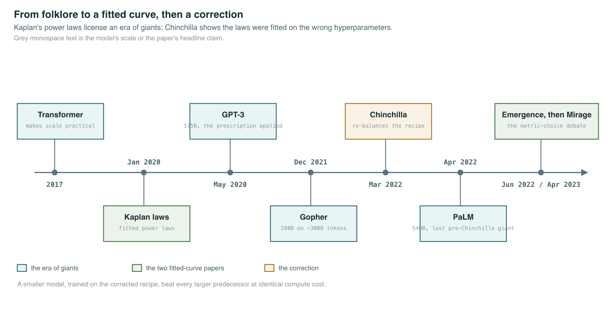
Act one: the power laws. “Scaling Laws for Neural Language Models” (Kaplan et al., 2020), submitted in January 2020, trained families of transformer language models across many sizes and measured how the cross-entropy loss (the quantity introduced in chapter 1) fell as three resources grew: non-embedding parameters, dataset tokens, and training compute. The result was startlingly clean. Loss followed smooth power laws in each variable, “with some trends spanning more than seven orders of magnitude.” Architecture details — depth versus width, number of heads — mattered far less than raw scale. For the first time, a lab could train a sweep of small models, fit three constants, and read off the expected loss of a model a thousand times larger.

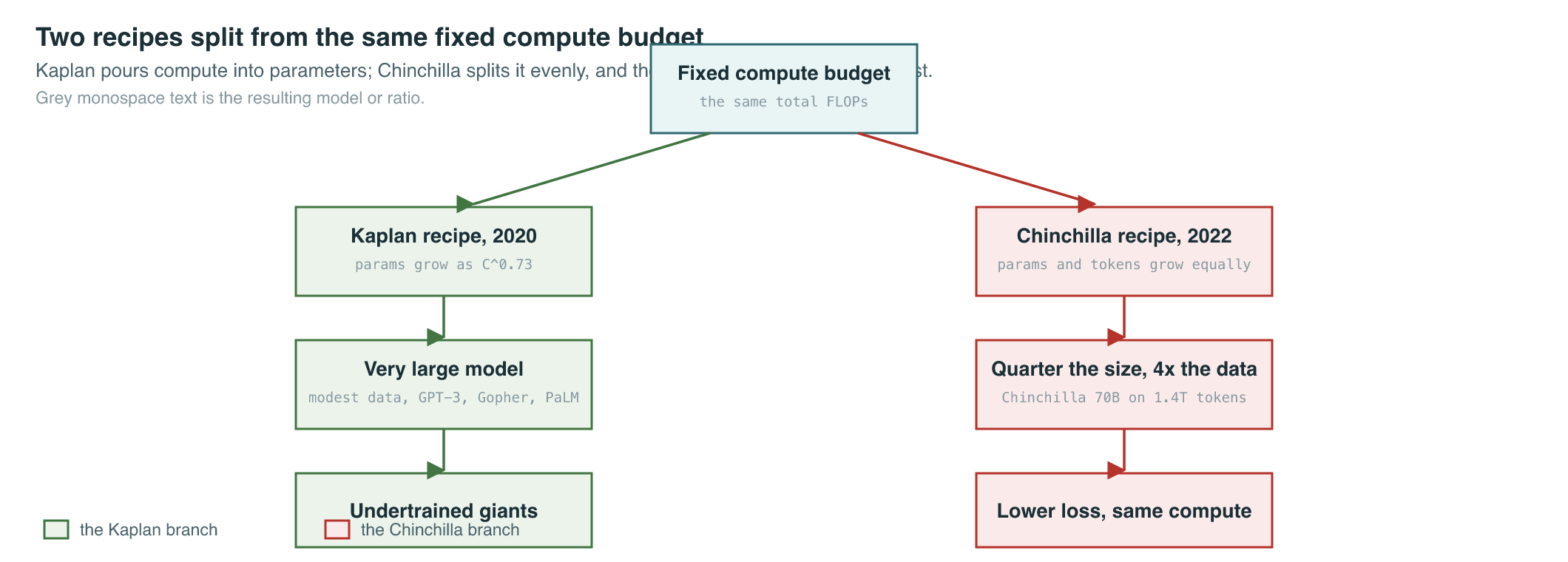
The paper’s most consequential claim was about allocation. Larger models were found to be significantly more sample-efficient, so “optimally compute-efficient training involves training very large models on a relatively modest amount of data and stopping significantly before convergence.” Concretely, as the compute budget grew, parameters should grow much faster than data. The field listened. GPT-3 (Brown et al., 2020), submitted in May 2020, was a 175-billion-parameter model — in its authors’ words, “10x more than any previous non-sparse language model” — and its headline result, few-shot in-context learning, is the subject of chapter 7. Gopher (Rae et al., 2021), DeepMind’s 280-billion-parameter model of December 2021, trained on roughly 300 billion tokens. PaLM (Chowdhery et al., 2022), Google’s April 2022 system, trained a 540-billion-parameter dense transformer on 780 billion tokens. The era of giants was a direct application of the Kaplan prescription: enormous parameter counts, comparatively little data.

Act two: the correction. “Training Compute-Optimal Large Language Models” (Hoffmann et al., 2022), submitted in March 2022, re-ran the measurement with one methodological fix. The Kaplan sweep had used, in Hoffmann et al.’s words, “a fixed number of training tokens and learning rate schedule for all models; this prevents them from modelling the impact of these hyperparameters on the loss.” When the learning-rate schedule is matched to the actual token budget of each run, the picture changes. Training over 400 models from 70 million to over 16 billion parameters on 5 to 500 billion tokens, the DeepMind team found that “for every doubling of model size the number of training tokens should also be doubled” — parameters and data should scale equally with compute, not with parameters far ahead.

By that arithmetic, every headline model of the previous two years was substantially undertrained: too many parameters, too few tokens. The proof was empirical. Chinchilla, a 70-billion-parameter model trained on 1.4 trillion tokens — the same compute budget as Gopher, spent on a model a quarter the size seeing over four times the data — outperformed Gopher, GPT-3, and other larger models across a wide range of evaluations. On the MMLU benchmark it reached 67.5% average accuracy, more than 7 percentage points above Gopher. A smaller model, trained correctly, beat a bigger one at identical cost — and was cheaper to serve forever after.

One caveat both papers share: the laws were fitted on dense transformers. Sparse mixture-of-experts models decouple parameter count from per-token compute and follow their own accounting.

The Mathematics

Kaplan et al. found that when only one resource binds, test loss follows a power law in that resource:

$$\begin{aligned} L(N) &= \left(\frac{N_c}{N}\right)^{\alpha_N}, \quad \alpha_N \approx 0.076,\ N_c \approx 8.8 \times 10^{13} \\ L(D) &= \left(\frac{D_c}{D}\right)^{\alpha_D}, \quad \alpha_D \approx 0.095,\ D_c \approx 5.4 \times 10^{13} \\ L(C_{\min}) &= \left(\frac{C_c}{C_{\min}}\right)^{\alpha_C}, \quad \alpha_C \approx 0.050,\ C_c \approx 3.1 \times 10^{8} \end{aligned}$$

Symbol	Meaning
$L$	Cross-entropy test loss in nats per token
$N$	Non-embedding parameter count
$D$	Dataset size in tokens
$C_{\min}$	Minimum training compute in PF-days
$N_c, D_c, C_c$	Fitted scale constants for each law
$\alpha_N, \alpha_D, \alpha_C$	Fitted power-law exponents

From these laws Kaplan et al. derived how a growing compute budget should be split:

$$N \propto C_{\min}^{0.73}, \qquad B \propto C_{\min}^{0.24}, \qquad S \propto C_{\min}^{0.03}$$

Symbol	Meaning
$N$	Model parameters
$B$	Batch size
$S$	Number of training steps
$C_{\min}$	Minimum training compute (same quantity as in the laws above)

Hoffmann et al. replaced the single-variable laws with a joint parametric fit over both parameters and data:

$$L(N, D) = E + \frac{A}{N^{\alpha}} + \frac{B}{D^{\beta}}, \quad E \approx 1.69,\ A \approx 406.4,\ B \approx 410.7,\ \alpha \approx 0.34,\ \beta \approx 0.28$$

Symbol	Meaning
$E$	Irreducible loss floor, fitted at 1.69
$A, B$	Fitted constants weighting each penalty term
$\alpha, \beta$	Fitted exponents, 0.34 for parameters and 0.28 for data
$N$	Model parameters
$D$	Training tokens

Minimizing this loss subject to a fixed compute budget gives the compute-optimal allocation:

$$N_{\mathrm{opt}} \propto C^{a}, \qquad D_{\mathrm{opt}} \propto C^{b}, \qquad a \approx b \approx 0.5$$

Symbol	Meaning
$N_{\mathrm{opt}}$	Compute-optimal model parameter count
$D_{\mathrm{opt}}$	Compute-optimal training token count
$C$	Total training compute (FLOPs)
$a, b$	Fitted exponents, both approximately 0.5

Hoffmann et al. estimated the exponents three independent ways, and all three agreed:

Approach	$a$ (parameters)	$b$ (tokens)
1 — Fix model sizes, vary training tokens	0.50	0.50
2 — IsoFLOP profiles	0.49	0.51
3 — Parametric loss fit	0.46	0.54
Kaplan et al. (2020), for contrast	0.73	0.27

What It Enabled

The most direct legacy of the two papers is that frontier training runs became engineered rather than gambled. Scaling-law sweeps — train dozens of small models, fit the curve, commit the budget — became a standard line item in every serious pretraining effort, a practice detailed in training runs in practice. The tokens-per-parameter ratio became the fastest way to read a model announcement:

Model	Date	Parameters	Training tokens	Tokens per parameter
Gopher (Rae et al., 2021)	Dec 2021	280B	~300B	~1.1
Chinchilla (Hoffmann et al., 2022)	Mar 2022	70B	1.4T	20
PaLM (Chowdhery et al., 2022)	Apr 2022	540B	780B	~1.4
Llama 3 405B (Grattafiori et al., 2024)	Jul 2024	405B	15.6T	~39

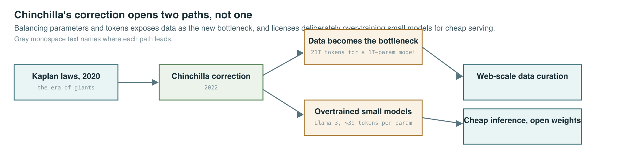
The second legacy was to move the bottleneck. If data must scale with parameters, then data — not hardware — becomes the binding constraint. Hoffmann et al.’s own projections made this explicit: a compute-optimal 1-trillion-parameter model would need roughly 21.2 trillion training tokens, and the paper noted that “the amount of training data that is projected to be needed is far beyond what is currently used to train large models, and underscores the importance of dataset collection.” That warning is the opening premise of chapter 11, the data question.

The third legacy came after Chinchilla, and partially superseded it: over-training. Chinchilla optimizes training compute alone, but a model is trained once and served millions of times. Llama 3 (Grattafiori et al., 2024) made the trade explicit — its flagship 405B model sat near its own compute-optimal point at 15.6 trillion tokens, but Meta deliberately chose to “train our smaller models for much longer than is compute-optimal. The resulting models perform better than compute-optimal models at the same inference budget.” Small, heavily over-trained models are the economic engine of the open-weights explosion and of cheap API tiers, and the successor question — whether to spend marginal compute at training time or at inference time — is taken up in the economics of test-time compute and reasoning models.

The emergence debate. Scaling laws predict loss, not abilities — and the gap between the two produced the era’s sharpest scientific argument. “Emergent Abilities of Large Language Models” (Wei et al., 2022), submitted in June 2022, defined an ability as emergent if it is “not present in smaller models but is present in larger models,” and catalogued examples where task performance sat at random until a scale threshold, then jumped: three-digit arithmetic appearing in GPT-3 at roughly 2×10²² training FLOPs (about 13B parameters); MMLU performance surpassing random only at 3–5×10²³ FLOPs (70B–280B parameters); chain-of-thought prompting beating standard prompting only near 10²³ FLOPs (~100B parameters); instruction tuning hurting models of about 8B parameters or smaller while helping at ~100B. The unsettling implication was that smooth loss curves could hide discontinuous capability jumps — you could not know what the next scale-up would unlock, for good or ill.

The rebuttal arrived in April 2023. “Are Emergent Abilities of Large Language Models a Mirage?” (Schaeffer et al., 2023) argued that “emergent abilities appear due to the researcher’s choice of metric rather than due to fundamental changes in model behavior with scale.” Exact-match accuracy on a multi-digit arithmetic problem is all-or-nothing: a model whose per-digit accuracy improves smoothly will score zero until it crosses the threshold where every digit comes out right, then appear to leap. Swap the discontinuous metric for a continuous one — per-token error, edit distance — and, in the authors’ analysis of GPT-3 results and a meta-analysis of BIG-Bench claims, the sharp jumps flatten into the familiar smooth curves. The debate is not fully settled — some capability thresholds matter precisely because the real world grades with discontinuous metrics — but the Mirage paper permanently raised the evidentiary bar for claims that scale produces qualitative surprises.

Key Papers

Paper	Authors	Year	Link	Why it matters
Scaling Laws for Neural Language Models	Kaplan et al.	2020	arXiv:2001.08361	First clean power laws for LM loss; made scale a predictable engineering variable
Language Models are Few-Shot Learners	Brown et al.	2020	arXiv:2005.14165	GPT-3 at 175B — the Kaplan prescription executed at full size
Scaling Language Models: Methods, Analysis & Insights from Training Gopher	Rae et al.	2021	arXiv:2112.11446	280B model on ~300B tokens; the undertrained baseline Chinchilla beat
Training Compute-Optimal Large Language Models	Hoffmann et al.	2022	arXiv:2203.15556	The Chinchilla re-balance: scale parameters and tokens equally
PaLM: Scaling Language Modeling with Pathways	Chowdhery et al.	2022	arXiv:2204.02311	540B dense model on 780B tokens; the last great pre-Chinchilla giant
Emergent Abilities of Large Language Models	Wei et al.	2022	arXiv:2206.07682	Named and catalogued discontinuous capability jumps with scale
Are Emergent Abilities of Large Language Models a Mirage?	Schaeffer et al.	2023	arXiv:2304.15004	Showed metric choice can manufacture emergence; reframed the debate
The Llama 3 Herd of Models	Grattafiori et al.	2024	arXiv:2407.21783	Deliberate over-training past Chinchilla-optimal for inference economics

PM Lens