RNNs, LSTMs, and seq2seq

It is September 2014. Word vectors can capture that Paris relates to France the way Rome relates to Italy, yet no neural network can reliably read an English sentence and write out its French translation. Within one year, two ideas separated by seventeen years — a memory cell designed in 1997 and an encoder–decoder framing published in 2014 — combine to make “sequence in, sequence out” the default shape of neural language processing.

Where We Were

The language models of chapter 1 predicted the next word from a fixed, short window of preceding words: n-gram counts, and later Bengio’s 2003 neural probabilistic language model, both truncated history at a hard boundary. The embeddings of chapter 2 — word2vec (January 2013) and its relatives — gave each word a fixed vector regardless of context, and gave sentences no representation at all. Language, however, is a sequence of arbitrary length in which the words at position 40 can depend on the words at position 2. A model whose input size is fixed cannot, even in principle, represent that.

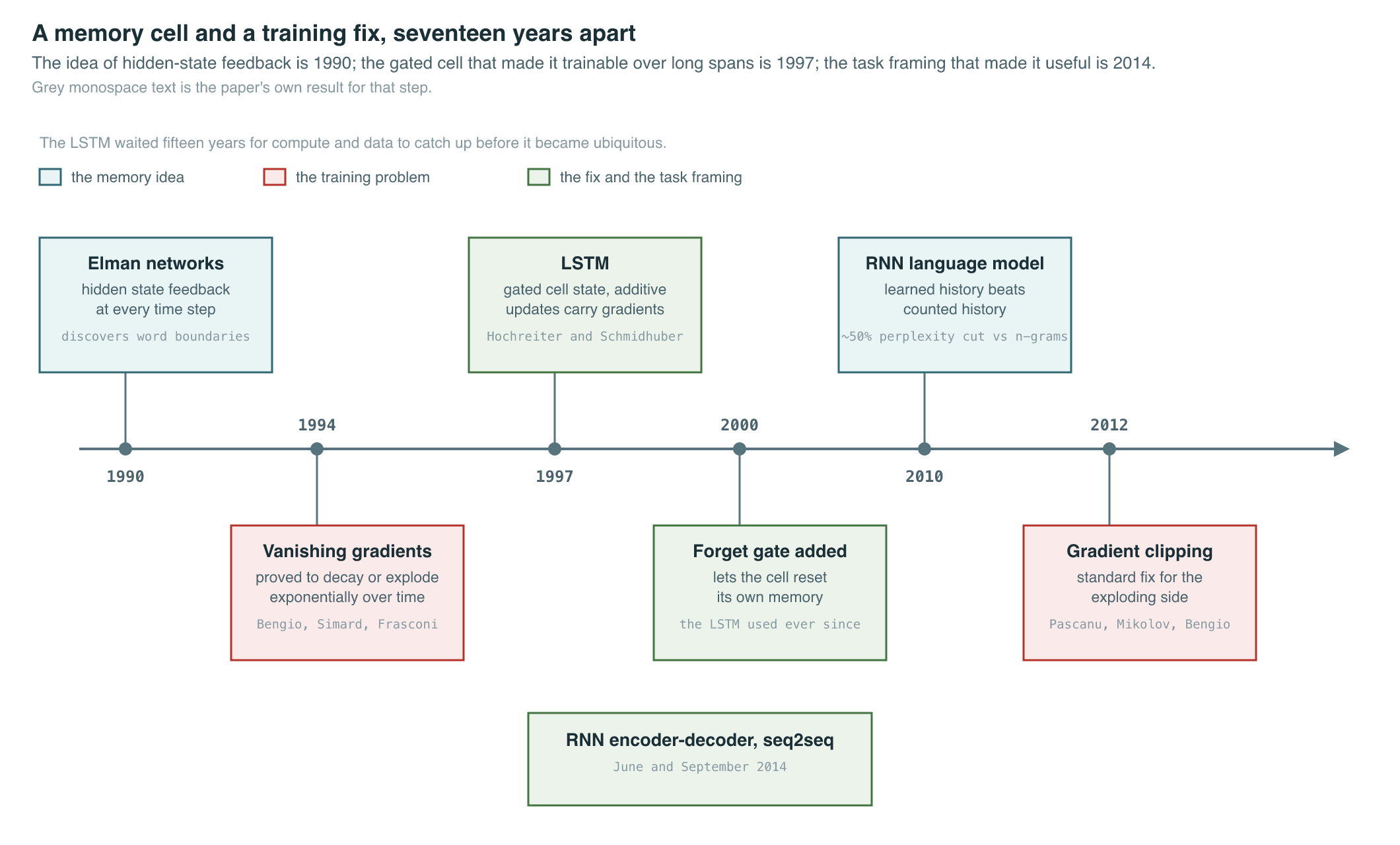
Recurrent neural networks were the obvious candidate architecture, and they were not new. Elman (1990) had described a “simple recurrent network” in which the hidden layer’s activations are fed back as input at the next time step, so the network maintains a state that summarizes everything it has read so far (Elman, 1990). Trained on letter and word sequences, Elman networks discovered word boundaries and rough syntactic categories — structure in time, as the title put it.

The problem was training them. Learning long-range dependencies requires propagating error signals backward through many time steps, and Bengio, Simard & Frasconi (1994) proved that this fails in a characteristic way: the gradient signal either decays exponentially toward zero or blows up exponentially as it travels back through time (Bengio et al., 1994). A network could learn dependencies spanning five or ten steps, but not fifty. Nearly two decades later, Pascanu, Mikolov & Bengio (2012) revisited the same pathology with modern tooling, gave it a geometric interpretation, and proposed the fix that became standard practice — clipping the gradient norm to handle explosions, plus a soft constraint to fight vanishing (Pascanu et al., 2012).

There were signs the approach could pay off despite the difficulty. Mikolov et al. (2010) trained recurrent language models for speech recognition and reported that a mixture of several RNN LMs cut perplexity by around 50% versus a state-of-the-art backoff n-gram model (Mikolov et al., 2010) — evidence that a learned, unbounded history beat counted, truncated history when you could get the training to work. What was missing was an architecture that made long-range credit assignment reliable, and a task framing that turned “language model” into “language transformer of input to output.”

The LSTM waited fifteen years for compute and data to catch up before it became ubiquitous; the idea was not late, the hardware was. PNG ↓

The Breakthrough

The breakthrough happened in two acts, seventeen years apart.

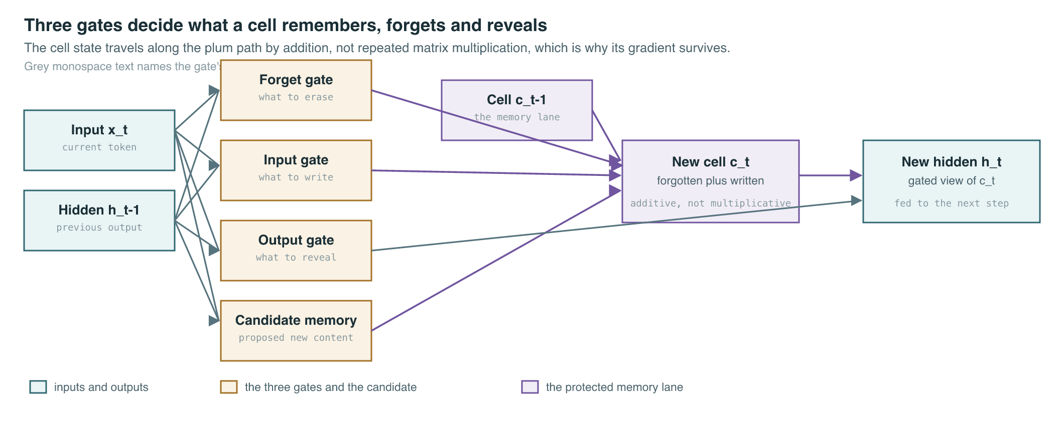
Act one: a cell that remembers. LSTM (Hochreiter & Schmidhuber, 1997) attacked the vanishing gradient at its source (Hochreiter & Schmidhuber, 1997). Instead of squashing the entire hidden state through a nonlinearity at every step, the long short-term memory unit maintains a separate cell state — a memory lane along which information can flow across time steps essentially unchanged, which the authors called the constant error carousel. Learned multiplicative gates decide, at each step, what enters this memory, what leaves it, and what is exposed to the rest of the network. Because the cell state is updated additively rather than by repeated matrix multiplication, error signals can travel backward across hundreds of steps without dying. Gers, Schmidhuber & Cummins (2000) completed the design with a forget gate that lets the cell learn to reset its own memory (Gers et al., 2000); the LSTM used in every system discussed below is this three-gate version.

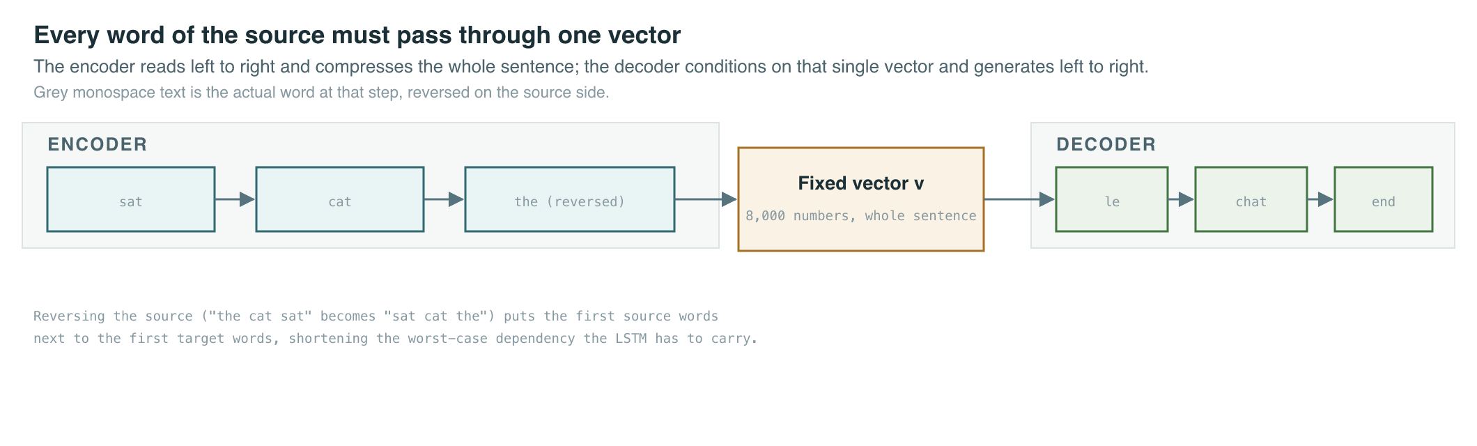
The cell state's path is dashed to mark it as additive, not repeated matrix multiplication, which is exactly the change that stops the gradient from vanishing. PNG ↓

Act two: two networks, one vector. For years the LSTM was applied where inputs and outputs aligned step-for-step — label each frame of audio, predict each next character. Translation does not align: an English sentence of 12 words may become a French sentence of 15, with word order scrambled. In June 2014, Cho et al. proposed the RNN Encoder–Decoder: one recurrent network reads the source sequence and compresses it into a single fixed-length vector; a second recurrent network conditions on that vector and emits the target sequence one symbol at a time (Cho et al., 2014). The same paper introduced a simplified gated unit — later named the gated recurrent unit, or GRU — that merged the LSTM’s gates into two. Cho’s system was still a component, not a replacement: the encoder–decoder scored phrase pairs as an extra feature inside a conventional statistical machine translation (SMT) pipeline.

Three months later, seq2seq (Sutskever, Vinyals & Le, September 2014) removed the pipeline entirely (Sutskever et al., 2014). A deep encoder — four LSTM layers of 1,000 cells each, with 1,000-dimensional word embeddings, 384M parameters in total — read the English sentence; a matching deep LSTM decoder generated the French translation token by token, trained end-to-end on the WMT’14 English-to-French corpus with a 160,000-word source vocabulary and an 80,000-word target vocabulary. On the WMT’14 test set the pure neural system scored 34.8 BLEU against 33.3 for a strong phrase-based SMT baseline — the first time an end-to-end neural model had beaten a mature SMT system on this benchmark — and reranking the SMT system’s 1,000-best lists with the LSTM pushed the score to 36.5.

One detail of the paper became folklore. The authors reversed the word order of every source sentence (but not the target), so that the first words of the input ended up adjacent to the first words of the output. This introduced many short-term dependencies between source and target and, in their words, made the optimization problem markedly easier. It is a telling artifact: even with LSTMs, the model strained to carry information across the full length of two concatenated sentences, and a data trick that shortened the worst-case dependency was worth real BLEU.

Reversing the source sentence puts its first words next to the target's first words, shortening the worst-case dependency the single vector has to carry. PNG ↓

The Mathematics

The vanilla recurrence. An Elman-style RNN maintains a hidden state $h_t$ updated at every time step:

h_t = \tanh\left(W_{hh}\, h_{t-1} + W_{xh}\, x_t + b_h\right)

Symbol	Meaning
$h_t$	hidden state (the network’s memory) at step $t$
$x_t$	input vector at step $t$ , e.g. a word embedding
$W_{hh}$	recurrent weight matrix, applied to the previous state
$W_{xh}$	input weight matrix, applied to the current input
$b_h$	bias vector
$\tanh$	elementwise squashing nonlinearity

Why gradients vanish. Training by backpropagation through time requires the derivative of a late state with respect to an early one, which is a product of one Jacobian per intervening step:

\frac{\partial h_t}{\partial h_k} \;=\; \prod_{i=k+1}^{t} \frac{\partial h_i}{\partial h_{i-1}} \;=\; \prod_{i=k+1}^{t} W_{hh}^{\top}\, \mathrm{diag}\!\left(\tanh'(a_i)\right)

To know how the state at step $t$ depends on the state at an earlier step $k$ , you multiply together one term for every step in between — each term being the recurrent matrix $W_{hh}$ times a diagonal matrix of $\tanh$ derivatives at that step’s pre-activation $a_i$ . Multiplying $t-k$ matrices together behaves like raising a number to the power $t-k$ : if the matrices tend to shrink vectors, the product collapses to zero (vanishing gradients — the model cannot learn long-range dependencies); if they stretch vectors, it explodes (training diverges). This is the result Bengio et al. formalized in 1994 and Pascanu et al. dissected in 2012; clipping the gradient norm handles the exploding side, but nothing in this architecture fixes the vanishing side. That required changing the recurrence itself.

Symbol	Meaning
$\partial h_t / \partial h_k$	sensitivity of the state at step $t$ to the state at step $k$
$\prod_{i=k+1}^{t}$	product of one factor per intervening time step
$W_{hh}^{\top}$	transpose of the recurrent weight matrix
$\mathrm{diag}(\tanh'(a_i))$	diagonal matrix of nonlinearity derivatives at step $i$
$a_i$	pre-activation entering the $\tanh$ at step $i$

The LSTM cell. The LSTM (with the forget gate of Gers et al., 2000) replaces the single squashed state with a gated cell state $c_t$ alongside the hidden state $h_t$ :

\begin{aligned} f_t &= \sigma\left(W_f x_t + U_f h_{t-1} + b_f\right) \\ i_t &= \sigma\left(W_i x_t + U_i h_{t-1} + b_i\right) \\ o_t &= \sigma\left(W_o x_t + U_o h_{t-1} + b_o\right) \\ \tilde{c}_t &= \tanh\left(W_c x_t + U_c h_{t-1} + b_c\right) \\ c_t &= f_t \odot c_{t-1} + i_t \odot \tilde{c}_t \\ h_t &= o_t \odot \tanh\left(c_t\right) \end{aligned}

Three gates — forget $f_t$ , input $i_t$ , output $o_t$ — are small learned dials between 0 and 1 (that is what the sigmoid $\sigma$ produces), each computed from the current input and the previous hidden state. The cell update line is the heart of the design: new memory $c_t$ equals old memory $c_{t-1}$ scaled by the forget gate, plus new candidate content $\tilde{c}_t$ scaled by the input gate, where $\odot$ means elementwise multiplication. Because old memory is carried forward by multiplication with a gate value that can sit near 1 — not by repeated passes through $W_{hh}$ and $\tanh$ — the gradient along the cell-state path neither vanishes nor explodes by default. What this buys you: dependencies spanning hundreds of steps become learnable, at the cost of roughly four times the parameters of a vanilla RNN of the same width.

Symbol	Meaning
$f_t, i_t, o_t$	forget, input, and output gates, each in the range 0 to 1
$\sigma$	logistic sigmoid, squashing to the range 0 to 1
$\tilde{c}_t$	candidate memory content proposed at step $t$
$c_t$	cell state — the protected long-term memory lane
$h_t$	hidden state — the gated, visible output of the cell
$W_\ast, U_\ast, b_\ast$	learned input weights, recurrent weights, and biases per gate
$\odot$	elementwise multiplication

Translation as conditional generation. seq2seq frames translation as modeling the probability of an output sequence given an input sequence. The encoder compresses the source $x_1, \ldots, x_T$ into a fixed-dimensional vector $v$ (its final hidden and cell states), and the decoder factorizes the output distribution one token at a time:

p\left(y_1, \ldots, y_{T'} \mid x_1, \ldots, x_T\right) \;=\; \prod_{t=1}^{T'} p\left(y_t \mid v,\; y_1, \ldots, y_{t-1}\right)

Symbol	Meaning
$x_1, \ldots, x_T$	source sequence, length $T$
$y_1, \ldots, y_{T'}$	target sequence, length $T'$ , generated left to right
$v$	fixed-dimensional encoding of the entire source sentence
$p(y_t \mid v, y_1, \ldots, y_{t-1})$	probability of the next token given the encoding and the tokens so far

What It Enabled

The most immediate effect was on machine translation itself. A discipline built over two decades — word alignment, phrase tables, log-linear feature weighting, separate language models — was matched by a single network trained end-to-end on sentence pairs.

	Phrase-based SMT, circa 2014	seq2seq NMT, September 2014
System shape	Pipeline of separately built components	One network, trained end-to-end
Linguistic knowledge	Hand-engineered features, alignment models	Learned from parallel text alone
Sentence representation	None — phrase-level statistics	One fixed vector per sentence
Handling of word order	Explicit reordering models	Implicit, learned by the decoder
WMT’14 En→Fr BLEU	33.3 (baseline reported in the paper)	34.8 direct; 36.5 reranking the SMT n-best lists
Vocabulary	Effectively open	Closed: 160k source, 80k target; unknown words penalized

The second effect was a template. “Encode the input, decode the output” turned out to fit almost any pair of sequences: summarization, dialogue, speech transcription, code generation. The generation loop that seq2seq established — produce one token, feed it back, produce the next — is, unchanged, how every modern chat model emits its answers.

The third effect was a well-defined failure to attack. All information about the source must pass through the single vector $v$ — 8,000 numbers in the Sutskever et al. system (four layers of 1,000 hidden and 1,000 cell units) — and translation quality degrades as sentences grow beyond what that bottleneck can hold; the sentence-reversal trick was a symptom, not a cure. In the same month seq2seq appeared (September 2014), Bahdanau et al. proposed letting the decoder look back at all encoder states and learn where to look — soft alignment, soon called attention. That mechanism, which dissolved the bottleneck and set up everything after it, is the subject of chapter 4.

The architecture’s remaining limits defined the next two chapters of research. The closed vocabulary problem — seq2seq penalized for every out-of-vocabulary word — was answered by subword tokenization (chapter 8). The strictly sequential computation — step $t$ cannot begin until step $t-1$ finishes, on both the time axis during training and across the eight GPUs of the original run — was answered by an architecture with no recurrence at all, the Transformer (chapter 5). Recurrence itself did not die so much as hibernate: state-space models revived the fixed-state, linear-time idea against attention’s quadratic cost a decade later (The Engine Room, chapter 18).

Recurrent unit	Gates	State carried	Key property
Elman RNN (1990)	none	$h_t$	Simplest recurrence; gradients vanish beyond short spans
LSTM (1997; forget gate 2000)	forget, input, output	$h_t$ and $c_t$	Additive cell-state path preserves gradients over long spans
GRU (2014)	update, reset	$h_t$	LSTM-like gating with fewer parameters, no separate cell state

Key Papers

Paper	Authors	Year	Link	Why it matters
Finding Structure in Time	Elman	1990	DOI	The simple recurrent network: hidden state as memory, structure discovered from sequence alone
Learning Long-Term Dependencies with Gradient Descent is Difficult	Bengio, Simard & Frasconi	1994	DOI	Proved gradients through time vanish or explode exponentially — the problem statement for a decade
Long Short-Term Memory	Hochreiter & Schmidhuber	1997	DOI	Gated cell state with additive updates; made long-range credit assignment learnable
Learning to Forget: Continual Prediction with LSTM	Gers, Schmidhuber & Cummins	2000	DOI	Added the forget gate, completing the LSTM as used everywhere since
Recurrent Neural Network Based Language Model	Mikolov et al.	2010	ISCA	A mixture of RNN language models cut perplexity ~50% versus backoff n-grams — recurrence beats counting
On the difficulty of training Recurrent Neural Networks	Pascanu, Mikolov & Bengio	2012	arXiv	Modern analysis of vanishing/exploding gradients; gradient norm clipping becomes standard
Learning Phrase Representations using RNN Encoder-Decoder for Statistical Machine Translation	Cho et al.	2014	arXiv	The encoder–decoder framing and the GRU; still a component inside an SMT pipeline
Sequence to Sequence Learning with Neural Networks	Sutskever, Vinyals & Le	2014	arXiv	End-to-end deep LSTM translation beats phrase-based SMT on WMT’14; the seq2seq template

PM Lens

What strikes me about seq2seq is how small the winning margin was: 34.8 BLEU versus 33.3, from a model that took ten days on eight GPUs and still couldn’t handle words outside an 80,000-word list. On the metric, that’s a modest win. On the roadmap, it was decisive — because the neural system was one trainable artifact where the SMT baseline was a pipeline of teams, and everyone could see which curve was still rising. I’ve watched the same call play out in ad tech: when an end-to-end learned system first ties the hand-tuned pipeline, the pipeline is already dead, because every future improvement on one side costs data and compute while on the other side it costs coordination across five owners. The other lesson is the reversal trick — a data-preprocessing hack worth real quality. Unglamorous input engineering routinely outperforms architecture work, and it still does; today we just call it data curation.

Search