From Shannon to n-grams

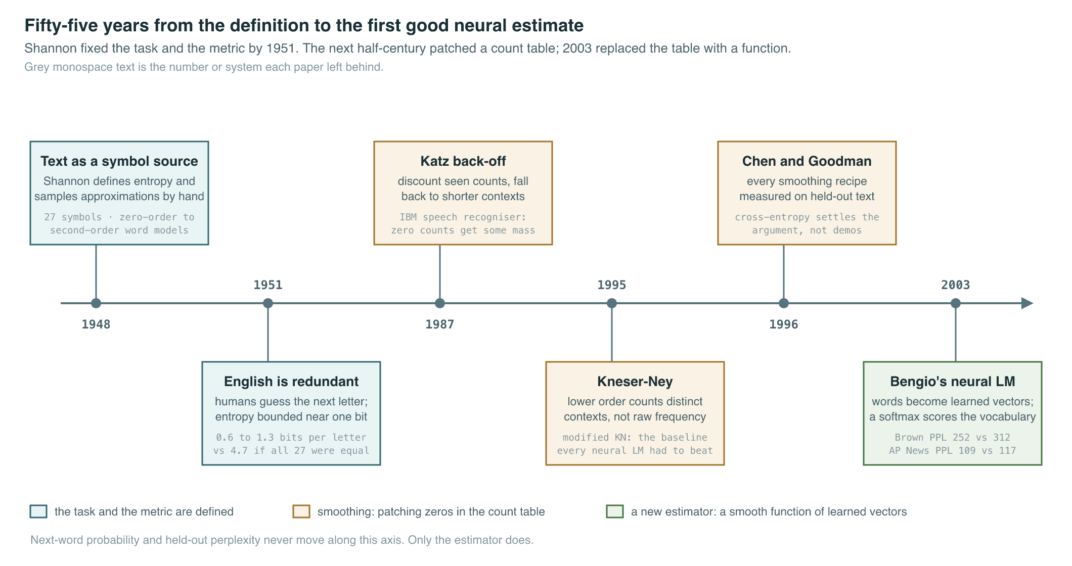
It is July 1948. In the Bell System Technical Journal, a 32-year-old Bell Labs mathematician named Claude Shannon publishes a two-part paper that treats English text not as grammar or meaning but as a stream of symbols emitted by a statistical process (Shannon, 1948). Every language model since — up to and including the systems that answer questions in complete paragraphs today — is an attempt to estimate the probability distribution Shannon defined in that paper. This chapter covers the fifty-five years it took to get from his definition to the first neural network that estimated it well.

Where We Were

Before 1948 there was no formal definition of the information content of a message, and no notion that predicting the next symbol of a text was a mathematically well-posed problem. Shannon’s A Mathematical Theory of Communication supplied both. He modeled a source of text as a discrete Markov process — a machine that emits symbols one at a time, where the probability of each symbol depends on the symbols that came before — and defined a single quantity, entropy, that measures how unpredictable the source is.

To show that this abstraction actually captures something about English, Shannon constructed what he called a “series of approximations to English,” using a 27-symbol alphabet of 26 letters plus the space. At each step, the generator respects more of the language’s statistics:

Zero-order approximation — symbols drawn independently and equiprobably: XFOML RXKHRJFFJUJ ZLPWCFWKCYJ.
First-order — symbols independent but drawn with English letter frequencies.
Second-order — each letter conditioned on the previous letter, using digram frequencies.
Third-order — each letter conditioned on the previous two, using trigram frequencies.
First-order word approximation — whole words drawn independently with their corpus frequencies.
Second-order word approximation — each word conditioned on the previous word: THE HEAD AND IN FRONTAL ATTACK ON AN ENGLISH WRITER THAT THE CHARACTER OF THIS POINT IS THEREFORE ANOTHER METHOD.

Shannon noted that “the resemblance to ordinary English text increases quite noticeably at each of the above steps.” Sampling from progressively better estimates of the next-symbol distribution produces progressively more convincing language. In 1948 the samples were constructed by hand, with tables of letter frequencies and a book opened at random. The observation, however, is the entire research program of generative language modeling stated in one sentence.

Three years later Shannon quantified how much structure there is to capture. In Prediction and Entropy of Printed English, he had human subjects guess the next letter of a text given the preceding context, and used their guess distributions to bound the entropy of printed English at roughly 0.6 to 1.3 bits per character (Shannon, 1951) — far below the 4.7 bits that 27 equiprobable symbols would carry. English is mostly redundant, which means it is mostly predictable, which means a machine that predicts it well is learning something real about the language.

The task and the metric were fixed by 1951 and never moved. Everything between then and 2003 is a better patch for the same count table; 2003 is the first time the table itself is replaced. PNG ↓

The n-gram decades

For the next several decades, the practical embodiment of Shannon’s idea was the n-gram model: approximate the probability of the next word using only the previous $n-1$ words, and estimate those probabilities by counting occurrences in a corpus. The main paying customer was speech recognition, where an acoustic model proposes candidate word sequences and a language model ranks them by plausibility — the setting named directly in the title of Katz’s IBM paper on estimating probabilities from sparse data (Katz, 1987).

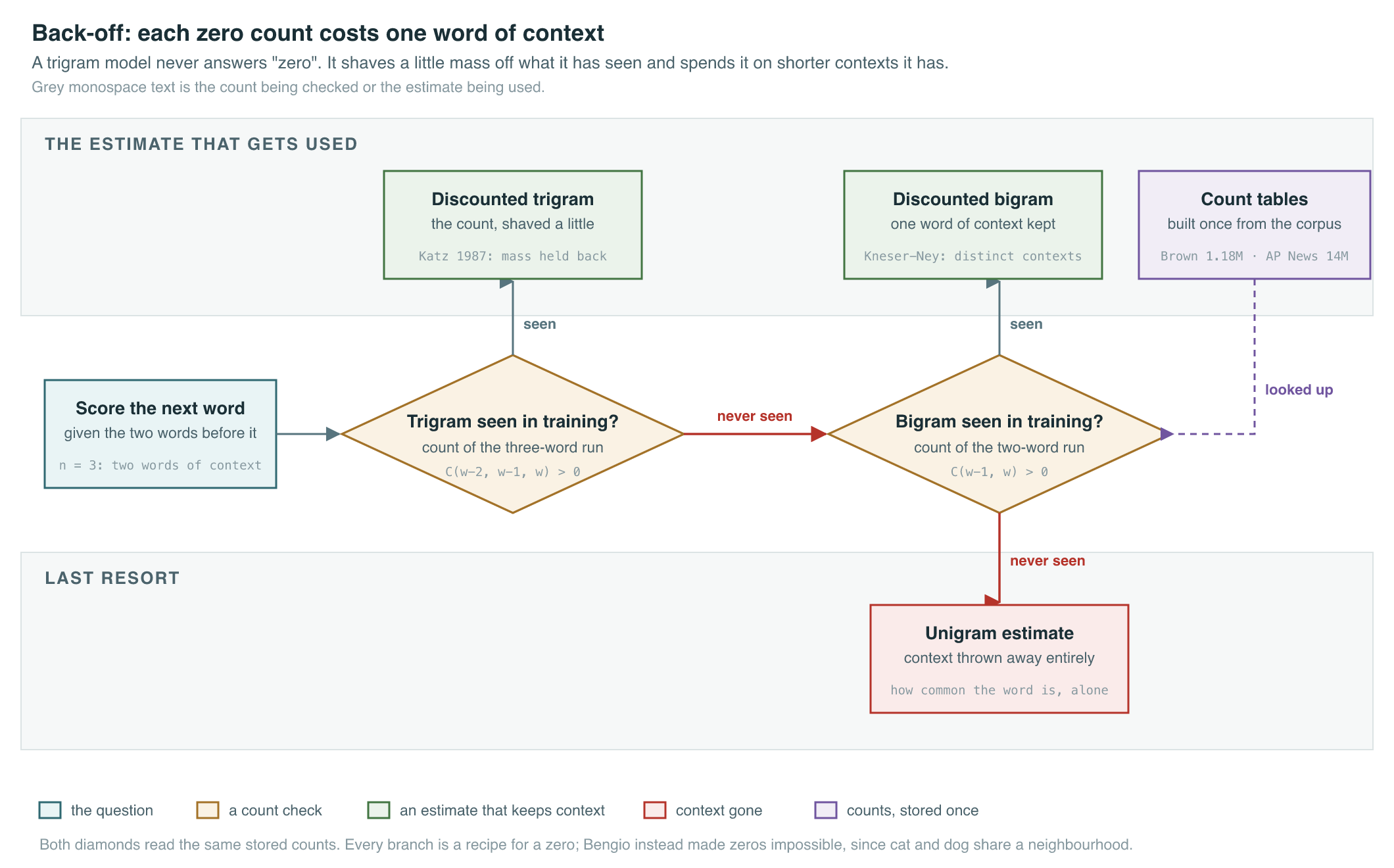
Counting works until it doesn’t. Most three-word sequences that a fluent speaker would accept never appear even once in any training corpus, and a naive count-based model assigns them probability zero — fatal when the model’s job is to score unseen sentences. The n-gram era’s central craft was therefore smoothing: systematically moving probability mass from seen events to unseen ones. Katz’s back-off scheme discounted observed counts and fell back to shorter contexts for unobserved ones (Katz, 1987). Kneser and Ney refined the back-off distribution itself, arguing that the lower-order estimate should reflect how many distinct contexts a word appears in rather than its raw frequency (Kneser and Ney, 1995). Chen and Goodman’s systematic empirical comparison of smoothing techniques, measured by held-out cross-entropy, put the whole subfield on a disciplined experimental footing (Chen and Goodman, 1996); the modified Kneser–Ney variant that emerged from that line of work became the standard baseline for a decade.

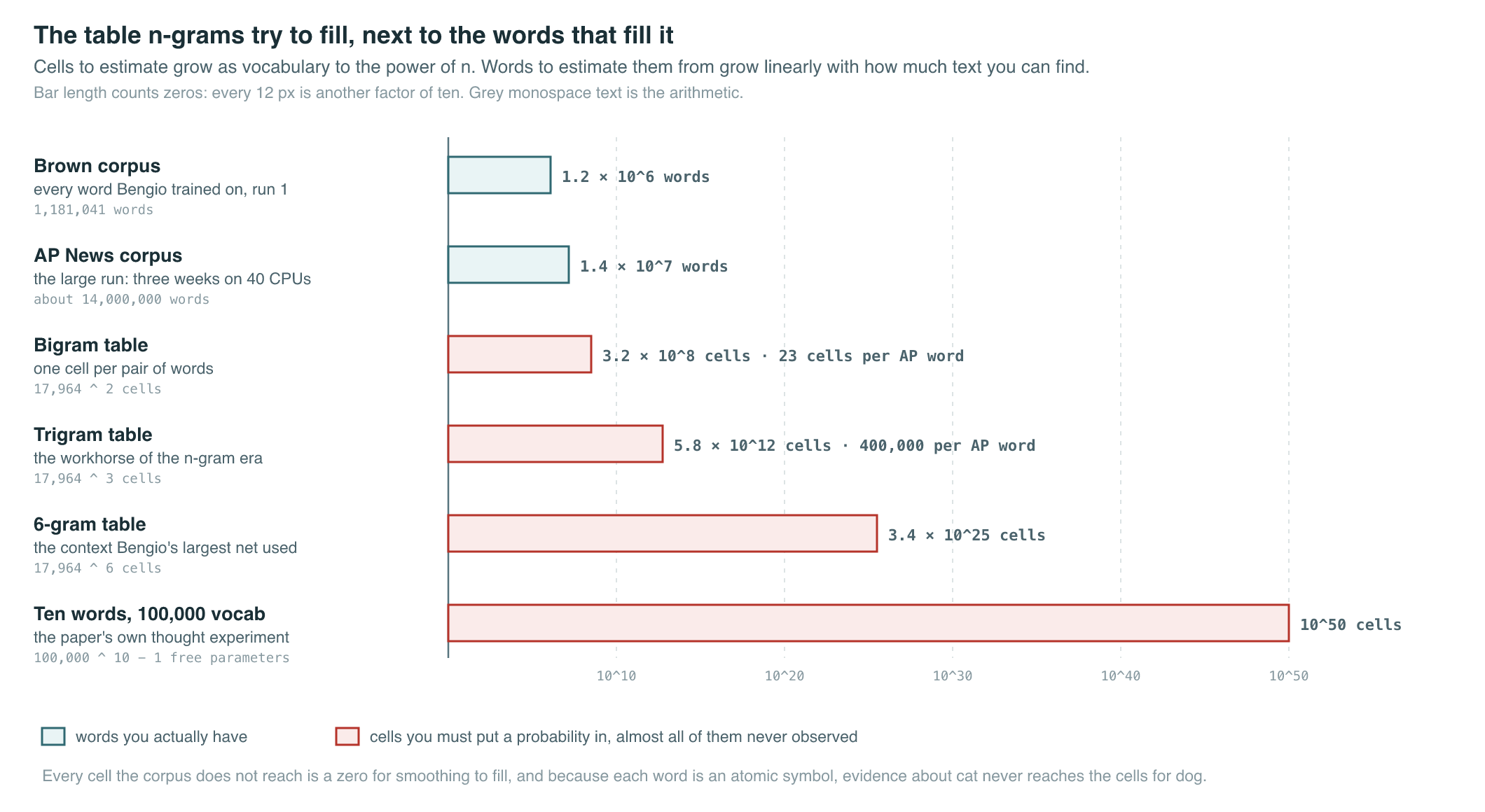
Back-off never returns zero, but each unseen count costs a word of context: the model that started with two words of history ends up scoring a word by how common it is on its own. PNG ↓

Smoothing treated the symptom, not the cause. The cause is what Bengio and colleagues would later call the curse of dimensionality: to model the joint distribution of 10 consecutive words over a vocabulary of 100,000, there are potentially $100000^{10} - 1 = 10^{50} - 1$ free parameters (Bengio et al., 2003). No corpus can populate that table. Worse, an n-gram model has no notion that cat and dog are similar words — each word is an atomic symbol, so evidence about sentences containing cat transfers nothing to sentences containing dog. Class-based n-grams (Brown et al., 1992) attacked this by grouping words into hand-counted clusters, a partial fix that hinted at the real answer: words needed representations with a geometry.

The corpus grows by finding more text; the table grows by the vocabulary raised to the power of n. Past the bigram row, almost every cell is a zero, and no amount of counting reaches it. PNG ↓

The Breakthrough

The breakthrough was published in February 2003 in the Journal of Machine Learning Research: A Neural Probabilistic Language Model by Yoshua Bengio, Réjean Ducharme, Pascal Vincent, and Christian Jauvin (Bengio et al., 2003). The paper made three moves that, taken together, defined the shape of every neural language model since:

Associate each vocabulary word with a learned, real-valued feature vector. Instead of an atomic symbol, a word becomes a point in a continuous space of $m$ dimensions — 30, 60, or 100 in the experiments, versus a vocabulary of roughly 17,000 words.
Express the probability of the next word as a smooth function of the feature vectors of the preceding words, computed by a neural network.
Learn the feature vectors and the network’s weights simultaneously, by maximizing the log-likelihood of the training corpus with stochastic gradient ascent.

The generalization argument is the heart of the paper. Because the probability function is smooth in the feature vectors, words that play similar roles are pushed toward similar vectors during training, and a small change in features produces a small change in predicted probabilities. Having seen a sentence about a cat, the model automatically assigns reasonable probability to the analogous sentence about a dog — one observed sentence informs a combinatorial neighborhood of unseen ones. Smoothing by geometry replaced smoothing by recipe.

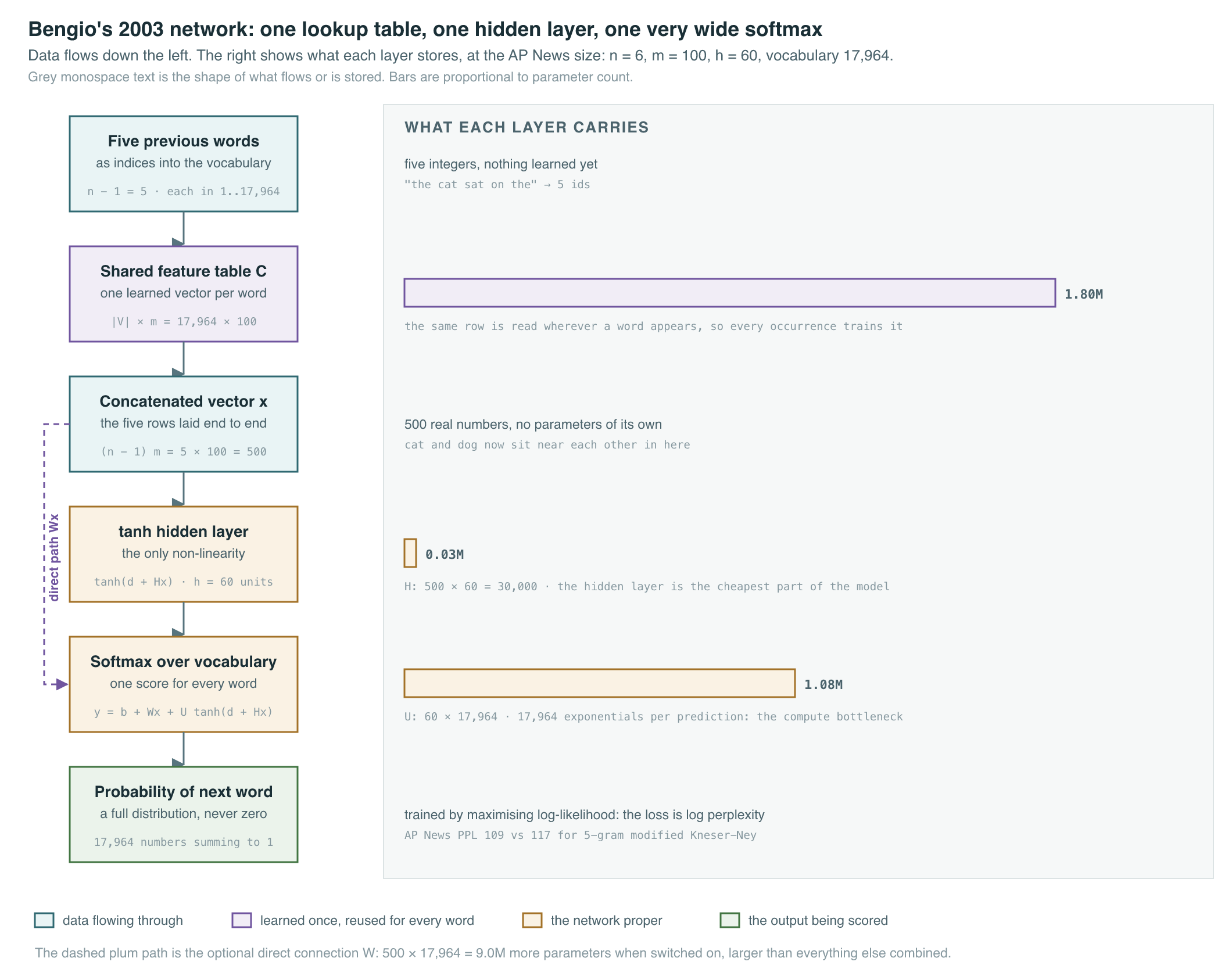
Almost every parameter sits in the two layers that touch the vocabulary: the lookup table on the way in and the softmax on the way out. The hidden layer that gives the model its name is the smallest thing in it. PNG ↓

The architecture is, by later standards, minimal: a shared embedding table, one hidden layer of tanh units, optional direct connections from the features to the output, and a softmax over the entire vocabulary. The largest configuration in the paper used an order of $n = 6$ — five words of context predicting the sixth — $h = 60$ hidden units, and $m = 100$ features per word over a vocabulary of 17,964 words.

The results were unambiguous. On the Brown corpus — a stream of 1,181,041 words with the vocabulary reduced to 16,383 types by merging rare words — the best neural model reached a test perplexity of 252, against 312 for the best n-gram baseline (a class-based model with 500 word classes) and 336 for a deleted-interpolation trigram: a 24 percent improvement over the strongest classical model. On the larger Associated Press news corpus (about 14 million training words from 1995–1996, vocabulary 17,964), the neural model scored 109 against 117 for a 5-gram modified Kneser–Ney back-off model — an 8 percent gain. Mixing the network’s predictions with an interpolated trigram helped in every configuration, evidence that the two model families fail in different places.

The price was compute. Training on AP News ran for only 5 epochs, and those 5 epochs took approximately three weeks on 40 CPUs, using a parallelized stochastic gradient scheme the authors engineered specifically because exchanging tens of megabytes of parameters between machines was prohibitively slow. An n-gram model on the same data was a counting exercise.

The Mathematics

Shannon’s entropy measures the average unpredictability of a symbol source:

H = -\sum_{i} p_i \log_2 p_i

A language model needs the probability of an entire sequence. The chain rule of probability factorizes it, with no approximation, into a product of next-word predictions — the same autoregressive factorization that later generated images pixel by pixel (taught in Pixels, One at a Time; here it is applied to words):

P(w_1, w_2, \dots, w_T) = \prod_{t=1}^{T} P(w_t \mid w_1, \dots, w_{t-1})

Symbol	Meaning
$w_t$	the word at position $t$ in the sequence
$T$	total number of words in the sequence
$P(w_t \mid w_1, \dots, w_{t-1})$	probability of the next word given all preceding words
$\prod_{t=1}^{T}$	product over every position in the sequence

The full conditioning history is unmanageable with counts, so an n-gram model truncates it to the previous $n-1$ words and estimates each factor by relative frequency:

\begin{aligned} P(w_t \mid w_1, \dots, w_{t-1}) &\approx P(w_t \mid w_{t-n+1}, \dots, w_{t-1}) \\ \hat{P}(w_t \mid w_{t-2}, w_{t-1}) &= \frac{C(w_{t-2}, w_{t-1}, w_t)}{C(w_{t-2}, w_{t-1})} \end{aligned}

Symbol	Meaning
$n$	order of the model — how many words of context, including the predicted one
$C(\cdot)$	count of a word sequence in the training corpus
$\hat{P}$	an estimate of the true probability, built from data
$w_{t-n+1}, \dots, w_{t-1}$	the truncated context window of $n-1$ preceding words

Evaluation uses perplexity, the exponentiated average negative log-probability the model assigns to a held-out text:

\mathrm{PPL} = 2^{-\frac{1}{T} \sum_{t=1}^{T} \log_2 \hat{P}(w_t \mid w_1, \dots, w_{t-1})}

Symbol	Meaning
$\mathrm{PPL}$	perplexity — effective number of equally likely next-word choices
$T$	number of words in the held-out test text
$\log_2 \hat{P}(\cdot)$	log-probability the model assigns to the correct next word
$2^{(\cdot)}$	converts average bits of surprise back into a branching factor

Bengio et al. replace the count table with a parametric function. Each context word is mapped through a shared feature matrix, the features are concatenated, passed through a hidden layer, and scored against every vocabulary word:

\begin{aligned} x &= \big(C(w_{t-1}), C(w_{t-2}), \dots, C(w_{t-n+1})\big) \\ y &= b + Wx + U \tanh(d + Hx) \\ \hat{P}(w_t = i \mid w_{t-1}, \dots, w_{t-n+1}) &= \frac{e^{y_i}}{\sum_{j} e^{y_j}} \end{aligned}

Line one: look up each of the $n-1$ context words in the shared table $C$ — one learned $m$ -dimensional vector per vocabulary word — and concatenate the results into $x$ . Line two: compute a raw score $y_i$ for every candidate next word, as the sum of a bias, an optional direct linear path from the features ( $Wx$ ), and a one-hidden-layer network ( $U \tanh(d + Hx)$ ). Line three: the softmax turns scores into a proper probability distribution. What this buys you is sharing: the matrix $C$ is the same for a word wherever it appears, so every occurrence of every word sculpts one common geometry — and that geometry, not the smoothing recipe, is what generalizes to unseen word combinations. Training maximizes the log-likelihood of the corpus, so the loss being minimized is exactly the quantity perplexity measures.

Symbol	Meaning
$C$	the $\lvert V \rvert \times m$ matrix of word feature vectors, learned jointly with the network
$x$	concatenation of the context words’ feature vectors, length $(n-1)\,m$
$H, d$	hidden-layer weights and biases; $h$ tanh units
$U$	hidden-to-output weights, one row of scores per vocabulary word
$W, b$	optional direct feature-to-output connections and output biases
$y_i$	unnormalized score for vocabulary word $i$

What It Enabled

The immediate, measurable win was perplexity. The durable win was the word feature vector — the idea that a word’s identity should be a learned point in a continuous space. A decade later, that single component was extracted, simplified, and scaled into word2vec (word2vec and the Geometry of Meaning), which made word embeddings a commodity and gave the field its first taste of arithmetic on meaning.

	n-gram model (1980s–1990s)	Neural probabilistic LM (2003)
Word representation	atomic symbol, no similarity structure	learned feature vector of 30–100 dimensions
Parameters	one per observed n-gram type	embedding table plus network weights; grows linearly with $n$
Unseen word combinations	probability from back-off and discounting recipes	generalization through vector-space similarity
Usable context	2–4 previous words in practice	5 previous words in the reported experiments
Best Brown-corpus test perplexity	312 — class-based, 500 classes	252 — a 24 percent improvement
AP News test perplexity	117 — 5-gram modified Kneser–Ney	109 — an 8 percent improvement
Training cost	counting and normalization	about three weeks on 40 CPUs for 5 epochs

Almost every limitation of the 2003 model names a later chapter of this book. The fixed context window of $n-1$ words could not model long-range dependencies; recurrent networks removed the fixed window (Recurrent Networks and seq2seq), and the Transformer later replaced recurrence with attention over the whole context (The Transformer). The softmax over every vocabulary word was the dominant computational cost, a bottleneck that pushed the field toward subword vocabularies (Tokenization). The observation that the larger corpus shrank the neural advantage from 24 to 8 percent was an early data point in the question of how model quality trades against data and compute — a question not answered rigorously until the scaling-law papers (Scaling Laws).

And the objective itself never changed. GPT-1, GPT-2, and GPT-3 maximize the same chain-rule log-likelihood with a bigger estimator (The GPT Lineage); their training loss is the log of the same perplexity Shannon’s framework defines. Shannon’s 1948 party trick — sample from the next-symbol distribution and watch the text get more convincing as the distribution improves — is, mechanically, what a modern chat model does at inference time.

Key Papers

Paper	Authors	Year	Link	Why it matters
A Mathematical Theory of Communication	Shannon	1948	doi	Defines entropy, models text as a Markov symbol source, and demonstrates the n-gram approximation series — the founding document of language modeling
Prediction and Entropy of Printed English	Shannon	1951	doi	Bounds the entropy of English near 1 bit per character via human prediction experiments — quantifying how much structure a model can learn
Estimation of Probabilities from Sparse Data for the Language Model Component of a Speech Recognizer	Katz	1987	doi	Back-off smoothing — the workhorse fix for zero counts that made n-gram models deployable in speech recognition
Improved Backing-Off for M-gram Language Modeling	Kneser and Ney	1995	doi	The smoothing method that, in modified form, became the strongest classical baseline — the number every neural LM had to beat
An Empirical Study of Smoothing Techniques for Language Modeling	Chen and Goodman	1996	arXiv	The systematic held-out comparison that standardized rigorous perplexity evaluation across smoothing methods
A Neural Probabilistic Language Model	Bengio et al.	2003	JMLR	First successful neural LM: learned word feature vectors plus a softmax over the vocabulary, beating the best n-grams by 24 percent on Brown

PM Lens

I find this the most commercially clarifying chapter in the book: the product every LLM vendor sells today is literally Shannon’s 1948 objective with a billing meter attached. When I compare API providers on per-token pricing, I am buying lower perplexity — nothing more exotic than that — and it keeps my vendor evaluations honest. Two habits from this era still pay my way. First, Chen and Goodman won arguments with held-out measurement, not demos; when a vendor shows me a cherry-picked transcript, I ask for the eval harness. Second, Bengio’s trade — 8 percent quality for three weeks on 40 CPUs versus an n-gram you could count in an afternoon — is the same cost-quality decision I make choosing between a frontier model and a small open-weights model for a feature. The 2003 paper looked economically absurd and was architecturally right; ChatGPT, launched November 2022, is that bet compounding for nineteen years. When the cheap method and the expensive method optimize the same metric, watch the expensive one’s cost curve.

Search