Pixels One at a Time

It is January 2016. GANs, introduced nineteen months earlier, can already produce sharp samples but assign no number to how likely any particular image is; VAEs assign a number but the images they produce from it are blurry. A team at Google DeepMind asks a narrower question: what if an image were treated exactly like a sentence — a sequence to be predicted one element at a time, left to right, top to bottom — and scored with the same exact likelihood that language models had used for decades?

Where We Were

By early 2016, two families of deep generative model existed side by side, and neither one gave a modeler both things a probabilistic model is supposed to offer: an actual density over images, and images that looked good when sampled. The VAE, introduced in 2013, trains a decoder against a tractable lower bound on log-likelihood — the ELBO, taught in full in Variational Autoencoders — but the Gaussian output assumption behind that bound systematically blurs fine detail, because a Gaussian likelihood penalizes a slightly-shifted sharp edge more than a globally blurred one. The GAN, introduced in 2014 and covered in The Adversarial Game, sidesteps density estimation entirely: a discriminator supplies a training signal without ever computing a likelihood, which is exactly why GAN samples in 2015 already looked sharper than VAE samples, and exactly why a GAN cannot tell you how probable a given image is, cannot detect an out-of-distribution input by its own score, and is not directly comparable across papers on a shared numeric scale.

Language modeling had been quietly running a different playbook the entire time. A sentence’s probability factorizes losslessly, term by term, via the chain rule of probability — an identity, not an approximation — into a product of next-word predictions, the exact mechanism this chapter teaches and that From Shannon to N-grams later applies to text. Recurrent language models of the early 2010s trained directly on that factorization, maximizing the exact log-likelihood of the training data with no bound, no adversarial proxy, and no blur term — because there is no output-distribution assumption to blur. The question a handful of papers began asking in 2015 and 2016 was simple: an image is a fixed, ordered grid of pixels, and a grid of pixels is a sequence, so why not model it the same way?

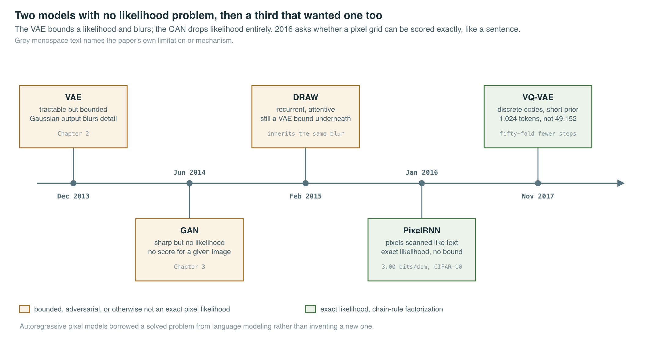
DRAW, a recurrent attention-based image generator published in February 2015 and taught in full in Variational Autoencoders, had already shown a network could generate an image through a sequence of attention-guided glimpses, but it optimized a VAE-style bound and inherited the same blur. What was missing was a model that kept the sequential, autoregressive machinery of a language model but pointed it at a pixel grid with no lower bound in the way — an exact, tractable density over full-resolution natural images, evaluated the same way a language model is evaluated: in bits, per symbol, on held-out data.

The Breakthrough

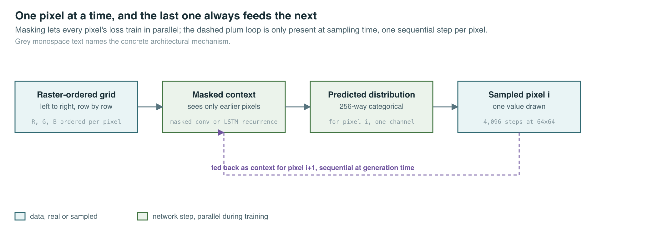
Pixel Recurrent Neural Networks (“PixelRNN”) (van den Oord et al., 2016) proposed exactly that: scan an image pixel by pixel, in raster order — left to right within a row, then row by row down the image — and predict each pixel’s distribution conditioned on every pixel that came before it in that scan order. Within a pixel, the three color channels are further ordered (red, then green, then blue), so the model predicts one scalar distribution at a time even inside a single pixel. The paper introduced two recurrent architectures to do this: a Row LSTM, which processes a row of pixels at a time using a one-dimensional convolution to combine information along the row, and a Diagonal BiLSTM, which re-skews the image so recurrence runs along diagonals, giving every pixel’s prediction access to an unbounded triangular context of everything above and to the left of it in a single pass in each of two directions. Both were paired with residual connections, letting the authors stack dozens of layers without the usual optimization difficulty of very deep recurrent stacks — the same problem residual connections had just solved, weeks earlier, for feedforward vision networks, per The Hardware Lottery’s account of ResNet.

The same paper described a third, purely convolutional variant: PixelCNN, which replaces recurrence with stacked convolutional layers whose receptive field is masked so that the filter computing pixel $i$ can see only pixels the raster order has already placed before $i$, never pixels after it. Masking, not recurrence, is what preserves the autoregressive property, and because masked convolutions can be evaluated in parallel across the whole image during training — every pixel’s loss computed in one forward pass, rather than one recurrent step per pixel — PixelCNN trained far faster than either LSTM variant, at a small cost in modeling quality: on CIFAR-10, the Diagonal BiLSTM reached 3.00 bits per dimension against PixelCNN’s 3.14, with Row LSTM in between at 3.07. The paper’s ImageNet 32×32 and 64×64 experiments used only the Row LSTM architecture, the first published likelihood benchmarks on that dataset.

Five months later, Conditional Image Generation with PixelCNN Decoders (“Gated PixelCNN”) (van den Oord et al., 2016) closed most of the quality gap while keeping the speed advantage. It made two changes to the original architecture. First, it replaced PixelCNN’s plain masked convolutions with gated convolutional layers — a multiplicative gate, borrowed from LSTM-style gating, applied inside each convolutional block — which closed most of the modeling-quality gap to the LSTM variants. Second, it removed the masked convolution’s receptive-field blind spot (a wedge of already-seen pixels that the original mask couldn’t attend to) by splitting each layer into two convolutional stacks, one conditioning on the current row and one on all rows above, combining their outputs after every layer. Together these changes let a purely convolutional model match Row LSTM’s log-likelihood on ImageNet (3.83 bits/dim at 32×32, 3.57 at 64×64, against Row LSTM’s 3.86 and 3.63) in under half the wall-clock training time: 60 hours on 32 GPUs, by the paper’s own account. It also added a second, orthogonal contribution: a conditioning vector — a class label, or an embedding produced by another network — added into every gated layer, so the same architecture that generated unconditional ImageNet samples could be steered to generate a requested class, or interpolate between two people’s face embeddings. That conditioning mechanism is the direct ancestor of every later “condition a generative model on an external vector” pattern this book covers, from class-conditional GANs to text-conditioned diffusion.

Autoregressive pixel models had one structural cost that no amount of architecture tuning removed: sampling is inherently sequential. Training could be parallelized across every pixel of every image in a batch, because during training the correct previous pixels are already known from the data. Generation cannot: pixel $i$‘s distribution depends on the sampled value of pixel $i-1$, which does not exist until it has itself been sampled, so producing one image at 64×64 resolution requires 4,096 sequential network evaluations, one per pixel, each waiting on the last. That sequential-generation cost — fine for language, where a sentence is already a modest-length sequence, brutal for a full-resolution image with tens of thousands of pixels — is the single biggest reason this family did not become the dominant way to generate images at scale, and it is the problem the next major idea in this chapter works around, not by making sampling faster, but by making the sequence shorter.

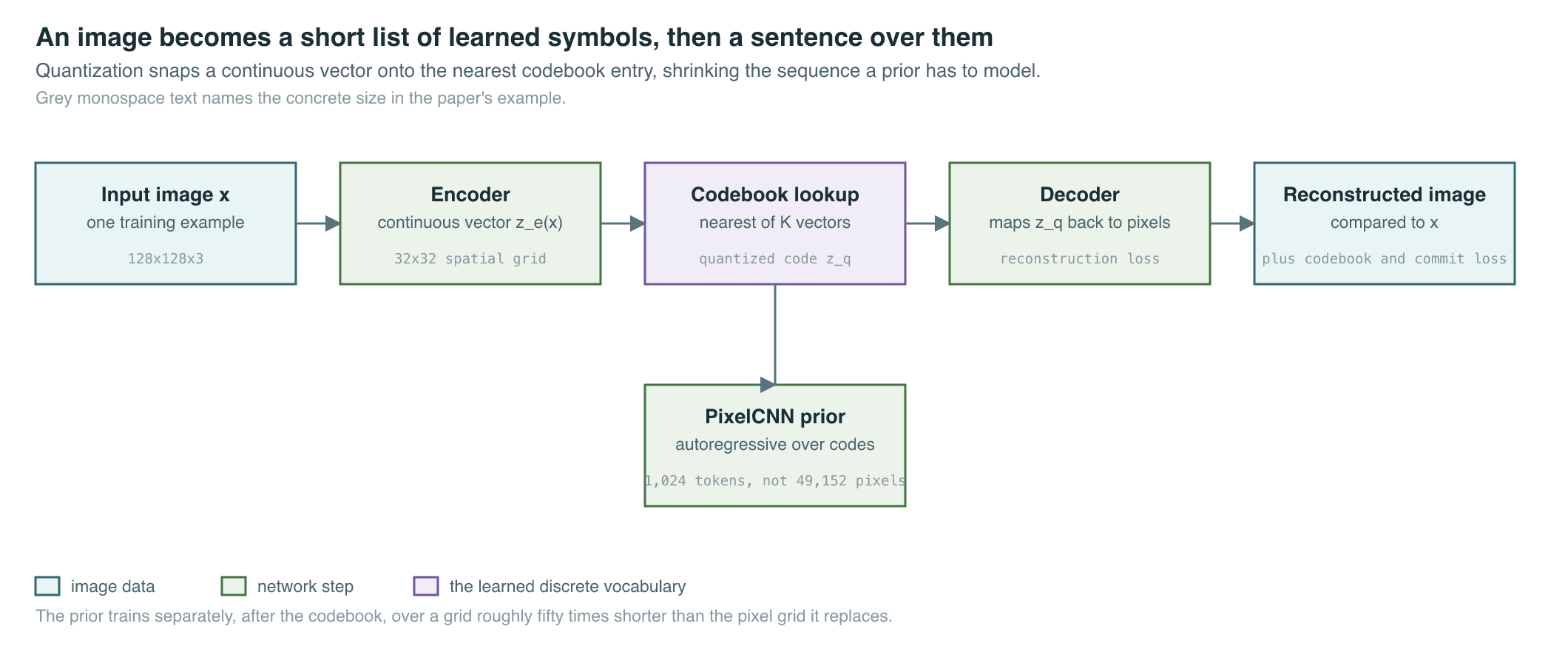
Neural Discrete Representation Learning (“VQ-VAE”) (van den Oord et al., 2017) reframed the same DeepMind team’s autoregressive machinery around a much smaller sequence. Instead of running a PixelCNN over raw pixels, VQ-VAE first learns an encoder that compresses an image into a small spatial grid of continuous vectors, then snaps — quantizes — each vector to the nearest entry in a learned, finite codebook of embedding vectors, producing a grid of discrete indices instead of raw pixels. A decoder reconstructs the image from the quantized grid. A PixelCNN prior is then trained, separately, over that much shorter grid of discrete codes rather than over pixels directly: for a 128×128×3 image encoded down to a 32×32×1 grid of codes, the autoregressive prior samples 1,024 discrete tokens instead of 49,152 pixel values, roughly a fifty-fold reduction in sequential sampling steps for that configuration. The idea of first learning a small, discrete vocabulary for images and then running an autoregressive model over that vocabulary — rather than over pixels — is the single largest lineage this chapter feeds into the rest of the book, traced in full below.

The Mathematics

An autoregressive model over an image $x$ with $n$ pixels, ordered $x_1$ through $x_n$ by the chosen raster scan, factorizes the joint distribution with the chain rule of probability — an exact identity, with no approximation and no lower bound:

$$p(x) = \prod_{i=1}^{n} p\big(x_i \mid x_1, \dots, x_{i-1}\big)$$

Each factor $p(x_i \mid x_1, \dots, x_{i-1})$ is what PixelRNN and PixelCNN actually parameterize with a neural network: given everything the raster order has already revealed, output a categorical distribution over the 256 possible values of the next pixel channel, then train by maximizing the log-likelihood the network assigns to the true next value, summed over every pixel of every training image — exactly the cross-entropy loss a language model trains against, applied to pixel intensities instead of vocabulary tokens.

VQ-VAE’s contribution is a different equation: how to snap a continuous encoder output onto the nearest of $K$ learned codebook vectors, and how to get a gradient through an operation — nearest-neighbor lookup — that has zero gradient almost everywhere. Quantization itself is a lookup:

$$z_q = e_k, \quad k = \arg\min_j \; \lVert z_e(x) - e_j \rVert_2$$

The full training objective combines a reconstruction term with two terms that manage the codebook, using the straight-through estimator to route gradients around the non-differentiable lookup:

$$\mathcal{L} = \underbrace{\lVert x - D(z_q) \rVert_2^2}_{\text{reconstruction}} \;+\; \underbrace{\lVert \operatorname{sg}[z_e(x)] - e_k \rVert_2^2}_{\text{codebook loss}} \;+\; \beta \underbrace{\lVert z_e(x) - \operatorname{sg}[e_k] \rVert_2^2}_{\text{commitment loss}}$$

Symbol	Meaning
$x$	An image, or a training example generally
$z_e(x)$	The encoder’s continuous output vector for $x$
$e_j$	The $j$-th vector in the learned codebook, $j = 1, \dots, K$
$z_q$	The quantized latent, the nearest codebook vector to $z_e(x)$
$D(\cdot)$	The decoder, mapping a quantized latent back to image space
$\operatorname{sg}[\cdot]$	Stop-gradient: identity on the forward pass, zero gradient on the backward pass
$\beta$	Weight on the commitment loss

On CIFAR-10, the original VQ-VAE paper trained a continuous VAE, VQ-VAE, and VIMCO baseline under the same setup and reported 4.51, 4.67, and 5.14 bits per dimension respectively — VQ-VAE cost about 0.16 bits/dim relative to the continuous VAE, a small likelihood penalty paid in exchange for a latent space that a discrete autoregressive prior can model at all.

What It Enabled

The immediate comparison the field drew was between exact-likelihood autoregressive models and the GAN/VAE alternatives already on the table, and the trade was stark: autoregressive pixel models delivered the best likelihoods of any image model at the time, at the cost of slow sequential sampling, while GANs delivered fast, sharp sampling with no likelihood at all.

Property	PixelRNN / PixelCNN, 2016	Contemporary GAN, 2016	VAE, 2013
Exact log-likelihood	Yes	No	Lower bound only
Sample sharpness (contemporary account)	Sharp, slow to produce	Sharp, fast to produce	Blurry
Sampling cost per image	One sequential network call per pixel	One forward pass	One forward pass
Trainable end to end	Yes, standard backprop	Yes, adversarial min-max	Yes, via the reparameterization trick
CIFAR-10 bits/dim (best variant reported)	3.00, Diagonal BiLSTM	Not directly comparable	4.51, comparable continuous VAE

A third family arrived alongside this lineage rather than descending from it: normalizing flows. Glow (Kingma and Dhariwal, 2018) built a generative model from a stack of invertible transformations — including a novel invertible 1×1 convolution — that maps data to a simple latent distribution and back, exactly, in both directions, using the change-of-variables formula to compute an exact log-likelihood without any sequential pixel-by-pixel scan and without a discriminator. Flows traded PixelCNN’s slow serial sampling for an architectural constraint of their own — every layer must be exactly invertible, which restricts the space of usable network designs — and never matched autoregressive or, later, diffusion likelihoods on natural images at scale, but they demonstrated that exact likelihood and one-shot (non-sequential) sampling were not mutually exclusive goals, a lesson the field returned to when building faster diffusion samplers, taught in Scores, SDEs, and Faster Sampling.

VQ-VAE’s discrete-codebook idea, not the pixel-by-pixel scan itself, is what carried furthest. Replacing VQ-VAE’s convolutional decoder with an adversarial one and its plain reconstruction loss with a perceptual and adversarial one produced VQGAN, whose codebook became the token vocabulary for the latent-space diffusion models covered in Latent Diffusion and Stable Diffusion. Running a large transformer, rather than a PixelCNN, as the autoregressive prior over a similar discrete codebook is the architecture behind DALL-E, covered in DALL-E and GLIDE. The same codebook-plus-autoregressive-prior pattern, applied to video frames instead of single images, is VideoGPT, taught in Tokens for Video. And the same discrete-vocabulary idea that a codebook builds for pixels is, from the opposite direction, exactly what byte-pair encoding builds for text, as covered in Tokenization — two independent solutions to the same underlying problem: giving a categorical, autoregressive model a finite alphabet to predict over. Later autoregressive image work returned to modeling raw pixels or coarse-to-fine scales directly (VAR, covered in The Current Frontier), but the discrete-codebook branch is the one that fed the systems eventually deployed at scale.

Key Papers

Paper	Authors	Year	Link	Why it matters
Pixel Recurrent Neural Networks	van den Oord et al.	2016	arXiv:1601.06759	Introduced exact-likelihood, pixel-by-pixel autoregressive image modeling and the masked-convolution trick that later architectures reused
Conditional Image Generation with PixelCNN Decoders	van den Oord et al.	2016	arXiv:1606.05328	Gated convolutions closed most of the quality gap to recurrent variants at roughly half the training cost, and added external conditioning
Glow: Generative Flow with Invertible 1x1 Convolutions	Kingma & Dhariwal	2018	arXiv:1807.03039	A contemporaneous exact-likelihood alternative via invertible flows, trading sequential sampling for an invertibility constraint
Neural Discrete Representation Learning	van den Oord et al.	2017	arXiv:1711.00937	Introduced the VQ-VAE discrete codebook and straight-through estimator that underlie VQGAN, DALL-E, and video tokenizers

PM Lens