Scores, SDEs, and Faster Sampling

It is the last quarter of 2020. DDPM (Ho et al., 2020) has just shown that a stack of learned denoising steps can match the image quality of adversarial networks, but the mechanism is expensive to run: generating one sample means simulating a Markov chain of up to a thousand sequential network evaluations. Within eight weeks of each other, two papers reframe what a diffusion model actually is — one as a family of non-Markovian processes that share DDPM’s training objective but not its slow sampler, the other as a single continuous-time stochastic differential equation that DDPM and an earlier line of score-based models both turn out to be discretizations of. A third paper, arriving a few months later, tightens the noise schedule and loss itself. Together they turn diffusion from a proof of concept into something a product team could plausibly ship.

Where We Were

DDPM’s generative process is a fixed, Markovian chain: to produce an image, the model starts from pure noise and takes a reverse step at every one of $T$ timesteps, each step calling the same denoising network once. The paper that established this — covered in Chapter 8, which owns the forward-noising construction and the simplified denoising loss $L_{\mathrm{simple}}$ that DDPM trains on — used $T = 1{,}000$ . That is not a rounding choice; the reverse process is only accurate when each step removes a small enough amount of noise that a Gaussian approximation holds, and DDPM’s ablations showed sample quality degrading sharply once fewer steps were used with the same sampler. A thousand sequential network calls per image is a real cost: no caching, no batching across steps, and no way around it, because step $t-1$ ‘s input is step $t$ ‘s output.

This was not the first time score functions and iterative denoising had been connected. A separate line of work, noise-conditional score networks (Song and Ermon, 2019) — also covered in Chapter 8 — trained a network to estimate the gradient of the log data density (the score) at several noise levels and used that gradient in Langevin dynamics to sample, arriving at image quality comparable to early GANs without adversarial training. DDPM and this score-based line looked, on the surface, like two separate research programs: one derived from a variational bound on a probabilistic model, the other from score matching and Langevin sampling. Both were slow for the same underlying reason — both needed many small, sequential steps — but neither paper had shown the other why.

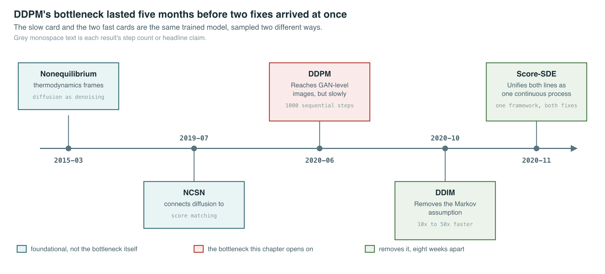
Two fixes for the same bottleneck landed within eight weeks of each other, sampling the same trained model two different ways. PNG ↓

By late 2020, the bottleneck was well understood even if the fix was not: whatever made diffusion sampling slow was tied to the assumption that the reverse process had to retrace the exact same discrete chain used in training, one small step at a time, with no way to skip ahead.

The Breakthrough

Denoising diffusion implicit models (Song, Meng, and Ermon, 2020) — DDIM — attacked the Markov assumption directly. The authors observed that DDPM’s training objective depends only on the marginal noising distribution at each timestep, not on the specific Markovian chain used to reach it. That leaves room to construct an entire family of non-Markovian forward processes that produce the exact same marginals, and therefore train with the exact same objective as DDPM, while having a different — and much more flexible — reverse process. One member of that family has a fully deterministic reverse map: given a noisy image at step $t$ , there is a unique output at any earlier step $t'$ , with no added noise in between. Because the reverse process no longer has to retrace every intermediate step to stay valid, it can jump across large gaps in the timestep sequence, generating a comparable image in a few dozen network calls instead of a thousand — the paper reports 10x to 50x wall-clock speedups over DDPM at matched quality. Determinism carries a second consequence: an image now has a single, fixed noise seed as its latent code, so two seeds can be interpolated and decoded into a smooth, semantically coherent path between two images — a capability the stochastic DDPM sampler does not offer.

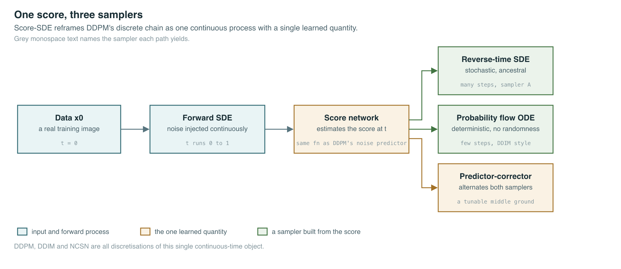
Score-based generative modeling through stochastic differential equations (Song et al., 2020) — Score-SDE — took a different route to a related destination. Rather than starting from DDPM’s discrete Markov chain, it modeled the forward noising process as a continuous-time stochastic differential equation (SDE): noise is injected continuously as time flows from $0$ to $1$ , not in a fixed number of discrete jumps. Every SDE has a corresponding reverse-time SDE that runs the noising process backward, and that reverse SDE depends on exactly one unknown quantity: the score of the noisy data distribution at each point in time — the same score that noise-conditional score networks had already been trained to estimate, and the same quantity DDPM’s noise-prediction network turns out to compute in disguise. That single observation unified both prior research programs: DDPM, DDIM, and score-based models are all discretizations of the same underlying object, differing only in the noising schedule and the sampler applied to it. The continuous-time view also produces a companion object with no randomness at all, the probability flow ODE, whose deterministic trajectories share the same marginal distributions as the stochastic reverse SDE — DDIM’s deterministic sampler is, in this framing, one particular discretization of this ODE.

One learned score function supports three samplers. DDPM, DDIM and NCSN are all discretisations of the same continuous-time object. PNG ↓

Improved denoising diffusion probabilistic models (Nichol and Dhariwal, 2021) came at the same problem from inside DDPM’s own discrete framework rather than by generalizing it. The paper made three changes: it let the reverse process learn its per-step variance instead of fixing it to a hand-set constant, it replaced DDPM’s linear noise schedule with a cosine schedule that destroys information more gradually near the end of the forward process, and it trained on a hybrid objective that mixes DDPM’s simple denoising loss with a small amount of the full variational bound, specifically to make the learned variances trainable without the noisy gradients that optimizing the full bound alone produces. The combined effect, per the paper’s own claim, was that learning the reverse-process variances allowed sampling with an order of magnitude fewer forward passes than the original fixed-variance sampler, at a negligible cost in sample quality — a result obtained without leaving DDPM’s discrete-time, Markovian formulation at all.

The Mathematics

DDIM’s deterministic sampling step reuses DDPM’s noise-prediction network $\epsilon_\theta$ but changes how successive steps are combined. Following DDIM’s own notation, where $\alpha_t$ denotes the cumulative noise-retention product Ho et al. call $\bar\alpha_t$ — the same quantity Chapter 8 writes with the bar; DDIM drops it:

x_{t-1} = \sqrt{\alpha_{t-1}}\left(\frac{x_t - \sqrt{1-\alpha_t}\,\epsilon_\theta(x_t, t)}{\sqrt{\alpha_t}}\right) + \sqrt{1-\alpha_{t-1}}\;\epsilon_\theta(x_t, t)

The term in parentheses is the network’s direct estimate of the clean image $x_0$ , built by removing the predicted noise $\epsilon_\theta(x_t, t)$ from the current noisy image $x_t$ and rescaling by $\sqrt{\alpha_t}$ . The equation then re-noises that estimate back up to exactly the noise level of step $t-1$ , using the same predicted $\epsilon_\theta(x_t, t)$ both times. Nothing random is drawn — every quantity on the right is a deterministic function of $x_t$ . What it buys you: because this update is a well-defined function of $x_t$ regardless of how far $t-1$ is from $t$ , $t-1$ can be tens of steps earlier than $t$ instead of exactly one step earlier, which is the entire mechanism behind DDIM’s speedup.

Symbol	Meaning
$x_t$	noisy image at timestep $t$
$x_{t-1}$	image at an earlier, not necessarily adjacent, timestep
$\alpha_t, \alpha_{t-1}$	cumulative noise-retention product at each timestep (DDIM’s notation for DDPM’s $\bar\alpha_t$ )
$\epsilon_\theta(x_t, t)$	network’s predicted noise, given the current noisy image and timestep

Score-SDE describes the forward noising process as a general Itô stochastic differential equation, of which DDPM’s discrete chain is one specific discretization:

\mathrm{d}x = f(x,t)\,\mathrm{d}t + g(t)\,\mathrm{d}w

Symbol	Meaning
$x$	the state (image) at time $t$ , evolving continuously
$t$	continuous time, running from data ( $t=0$ ) to noise ( $t=1$ )
$f(x,t)$	drift term, the deterministic part of the evolution
$g(t)$	diffusion coefficient, scaling how much noise is injected
$w$	standard Wiener process supplying the randomness

Every such forward SDE has a corresponding reverse-time SDE that undoes the noising, and it depends on exactly one learned quantity — the score:

\mathrm{d}x = \left[f(x,t) - g(t)^2 \,\nabla_x \log p_t(x)\right]\mathrm{d}t + g(t)\,\mathrm{d}\bar{w}

Symbol	Meaning
$x, t, f, g$	same roles as in the forward SDE, evaluated in reverse
$\nabla_x \log p_t(x)$	the score: gradient of the log density of noisy data at time $t$
$\bar{w}$	Wiener process running backward in time

Setting the noise term to zero gives a deterministic companion with the same marginal distributions at every $t$ — the probability flow ODE:

\mathrm{d}x = \left[f(x,t) - \tfrac{1}{2}g(t)^2 \,\nabla_x \log p_t(x)\right]\mathrm{d}t

Symbol	Meaning
$x, t, f, g$	same roles as in the forward SDE
$\nabla_x \log p_t(x)$	the score, here weighted by $\tfrac{1}{2}g(t)^2$ instead of the full $g(t)^2$ in the reverse SDE

The unification also explains why DDPM’s own noise-prediction network already had everything needed for a score-based sampler:

\nabla_x \log p_t(x_t) \approx -\frac{\epsilon_\theta(x_t, t)}{\sqrt{1-\bar\alpha_t}}

Symbol	Meaning
$\nabla_x \log p_t(x_t)$	the score at noise level $t$
$\epsilon_\theta(x_t, t)$	DDPM’s trained noise-prediction network
$\bar\alpha_t$	cumulative noise-retention product at timestep $t$

Improved DDPM’s cosine noise schedule replaces DDPM’s linear schedule for $\bar\alpha_t$ :

\bar\alpha_t = \frac{f(t)}{f(0)}, \qquad f(t) = \cos^2\!\left(\frac{t/T + s}{1+s}\cdot\frac{\pi}{2}\right), \qquad s = 0.008

Symbol	Meaning
$\bar\alpha_t$	cumulative signal-retention fraction at timestep $t$
$f(t)$	unnormalized cosine schedule function
$t, T$	current timestep and total number of timesteps
$s$	small offset preventing near-zero noise at $t=0$

Finally, the hybrid loss that makes learned variances trainable without destabilizing the mean prediction:

L_{\mathrm{hybrid}} = L_{\mathrm{simple}} + \lambda\, L_{\mathrm{vlb}}, \qquad \lambda = 0.001

Symbol	Meaning
$L_{\mathrm{hybrid}}$	combined training loss
$L_{\mathrm{simple}}$	DDPM’s original simplified denoising loss
$L_{\mathrm{vlb}}$	full variational lower bound, supplies the variance gradient
$\lambda$	small weight preventing $L_{\mathrm{vlb}}$ from dominating training

What It Enabled

The immediate effect was that diffusion stopped requiring a choice between “slow and stochastic” and “fast and low quality.” A single trained DDPM checkpoint could now be sampled with an ancestral sampler for maximum fidelity, or with DDIM for a fast preview, or with a predictor-corrector scheme for a middle ground — and Improved DDPM’s schedule and hybrid loss made the underlying network itself more sample-efficient no matter which sampler ran on top of it.

	DDPM sampler	DDIM sampler	Score-SDE (continuous)
Underlying process	discrete Markov chain	non-Markovian, same training loss as DDPM	continuous-time SDE / ODE
Typical steps to a good sample	up to 1,000	tens (10x–50x faster wall-clock than DDPM)	flexible; ODE solvers can adapt step size
Stochastic or deterministic	stochastic	deterministic (or a tunable blend)	either, via SDE or probability-flow ODE
Latent-space interpolation	not well-defined	yes, directly	yes, via the ODE
Reported result	GAN-competitive images (2020-06)	10x–50x speedup at matched quality	CIFAR-10 FID 2.20, Inception Score 9.89, 2.99 bits/dim; first 1024×1024 score-based samples

Score-SDE’s probability flow ODE also made exact likelihood computation tractable for the first time in this model family, via the standard change-of-variables formula for continuous normalizing flows — a capability score-based and DDPM-style models had lacked, and one that let researchers report bits-per-dimension numbers directly comparable to earlier likelihood-based generative models.

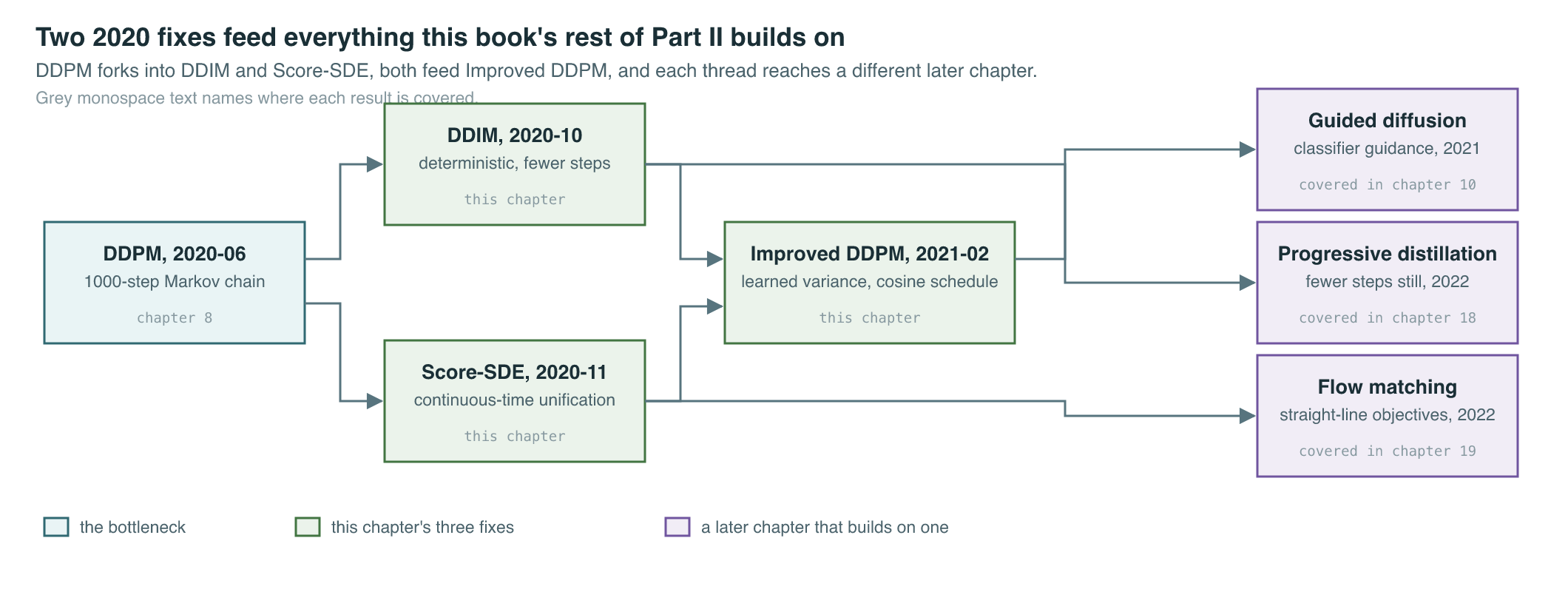
This chapter's three fixes are not a dead end. Guidance, few-step distillation and flow matching each pull a different thread forward. PNG ↓

The downstream lineage runs in two directions. Guided diffusion built directly on Improved DDPM’s architecture and added classifier guidance to trade diversity for fidelity, a technique generalized shortly after into classifier-free guidance — both covered in Chapter 10. Separately, DDIM’s demonstration that a fixed model tolerates a much shorter, custom sampling trajectory became the starting assumption for an entire later research thread on cutting sampling down further still, from tens of steps to a handful or to one, covered in Chapter 18. The probability flow ODE’s framing of generation as following a deterministic path from noise to data also generalizes into a broader family of straight-line and simulation-free training objectives, covered in Chapter 19. And once diffusion moved off pixels entirely, into the compressed latent spaces covered in Chapter 13, DDIM-style samplers became the default choice precisely because the per-step cost of an already-fast latent-space model made every additional step count.

Key Papers

Paper	Authors	Year	Link	Why it matters
Denoising Diffusion Implicit Models	Song, Meng, and Ermon	2020	arXiv:2010.02502	Removed the Markov assumption from DDPM’s sampler, cutting wall-clock sampling time 10x–50x and enabling deterministic latent-space interpolation
Score-Based Generative Modeling through Stochastic Differential Equations	Song et al.	2020	arXiv:2011.13456	Unified DDPM and score-based models as discretizations of one continuous-time SDE; introduced the probability flow ODE and exact likelihood computation
Improved Denoising Diffusion Probabilistic Models	Nichol and Dhariwal	2021	arXiv:2102.09672	Learned variances, a cosine noise schedule, and a hybrid loss cut required sampling steps by roughly an order of magnitude within DDPM’s own framework

PM Lens

This is the chapter I reach for whenever someone asks why an image-generation feature feels slow, or why a vendor’s quote for “high quality” mode costs several times more than its “fast” mode. Those two modes are, more often than not, the same trained model running two different samplers from this chapter — a 50-step DDIM path versus a slower stochastic one, or a coarser versus finer discretization of the same probability-flow ODE. Early Stable Diffusion (August 2022) shipped with roughly 50-step DDIM-family sampling as its default for exactly this reason: it was the cheapest setting that still looked finished. When I’m scoping a diffusion-based feature now, “which sampler, how many steps, what’s the quality-per-step curve” is a concrete engineering question with a real cost attached, not a vague quality dial — and every step you cut is GPU-seconds you don’t pay for on every single generation.

Search