Few-Step Generation

It is early 2022. Diffusion models already produce images that rival adversarial networks, and DDIM (Chapter 9) has already cut sampling from a thousand steps to a few dozen, but a few dozen sequential network calls is still far from the tens-of-milliseconds latency an interactive product needs. Over the next twenty months, four papers attack that remaining gap from four different angles — and by late 2023, the same class of model that once took a minute per image runs at a handful of steps, some of them fast enough for a live preview as a user types.

Where We Were

By 2022, a trained diffusion checkpoint could be sampled several different ways without retraining: an ancestral DDPM sampler for maximum fidelity, or DDIM (Chapter 9) for a faster, deterministic path through the same probability flow ODE. DDIM’s contribution was to show that the reverse process did not have to retrace every discrete step used in training — it could jump across gaps in the timestep schedule. That insight cut sampling from roughly a thousand steps to tens of steps, a 10x-to-50x wall-clock improvement, but it did not remove the sequential dependency itself: each of those tens of steps still had to wait on the output of the one before it, and each step was a full forward pass through a large denoising network.

Two other costs compounded the problem. First, classifier-free guidance (Chapter 10) — the technique that made text-to-image models actually follow their prompts — requires two network evaluations per step, one conditional and one unconditional, so a “20-step” guided sampler is closer to 40 network calls in practice. Second, once diffusion moved into the compressed latent spaces of latent diffusion and Stable Diffusion (Chapter 13), each individual step got cheaper, but the model itself — a large U-Net operating at high resolution — did not get faster to evaluate once per step. Multiplying a lower per-step cost by tens of guided steps still left a product with a multi-second wait between a prompt and a finished image, an experience closer to a batch job than to typing into a search box.

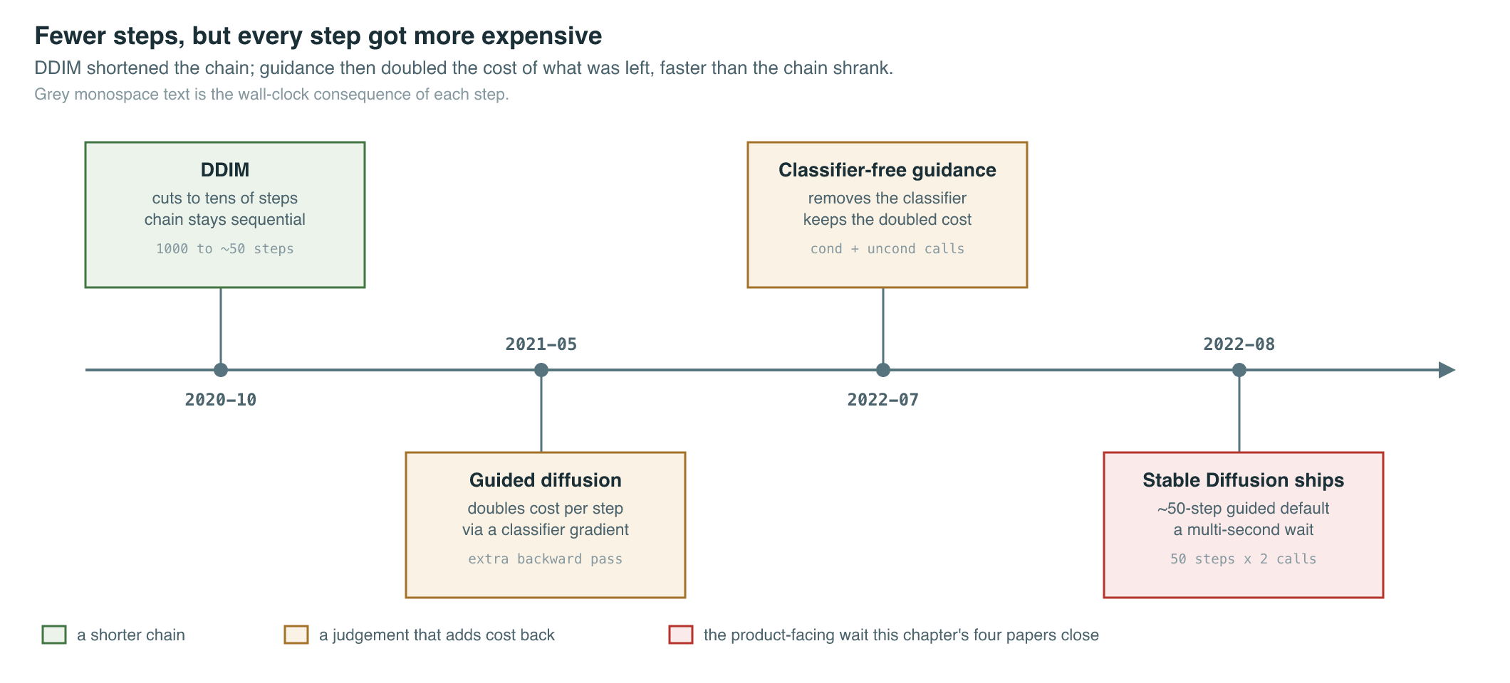
Sampler research through 2021 had focused on getting more image quality out of a fixed step budget — better ODE solvers, better noise schedules — rather than on asking whether the number of required steps could itself be trained down. That reframing, treating step count as a quantity a second training pass could optimize directly, is what the next four papers share, even though they arrive at it through different mechanisms.

The Breakthrough

Progressive distillation: halving the ladder. Tim Salimans and Jonathan Ho’s progressive distillation (Salimans and Ho, 2022) treated an already-trained diffusion model as a teacher and trained a student to match its output using half as many sampling steps. The student is not trained to imitate individual noise predictions; it is trained so that one student DDIM step reproduces the effect of two teacher DDIM steps in a row. Once that student matches its teacher, the student becomes the new teacher for a second round, halving the step count again — 1,024 steps to 512, to 256, and on down. The paper reports reaching as few as 4 sampling steps while keeping image quality competitive with the original many-step sampler, and the entire multi-round distillation procedure costs roughly the same compute as training the original model once, not once per round.

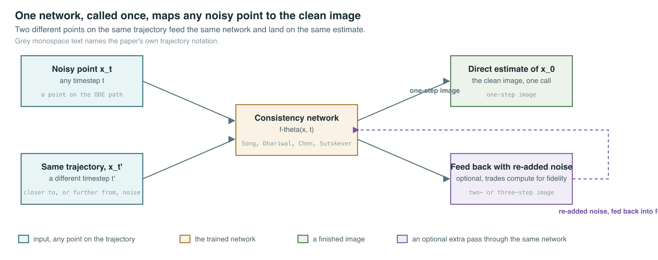
Consistency models: skip the ladder entirely. A year later, Yang Song, Prafulla Dhariwal, Mark Chen, and Ilya Sutskever asked whether a single network could learn to map any point on a diffusion trajectory directly to that trajectory’s starting point, in one function call, rather than learning to shorten a sequence of steps (Song et al., 2023). The probability flow ODE that DDIM and Score-SDE describe (Chapter 9) traces a deterministic path from a noisy point back to a clean image; consistency models train a network to output that same clean image no matter which point along the path it is given. Once trained, the network can produce a full image in a single forward pass — and, unlike progressive distillation’s fixed halving schedule, it can also be called two or three times, feeding its own output back in with a bit of re-added noise, to trade a small amount of extra compute for higher fidelity. The paper trains consistency models two ways: distilled from an existing pretrained diffusion model’s probability flow ODE, or trained as an independent generative model from scratch with no teacher at all, using an unbiased estimator of the same trajectory.

Latent consistency models: consistency meets text-to-image at scale. Consistency models were demonstrated on unconditional benchmarks — CIFAR-10, ImageNet, LSUN — not on guided, text-conditioned latent diffusion. Simian Luo, Yiqin Tan, Longbo Huang, Jian Li, and Hang Zhao closed that gap by distilling the consistency property directly into Stable Diffusion’s latent space, folding the classifier-free guidance scale into the trajectory itself rather than treating it as a separate doubled forward pass at sampling time (Luo et al., 2023). The resulting Latent Consistency Model (LCM) produces 768×768 images in two to four steps, and — because the guidance scale becomes an input the network conditions on during distillation, rather than a second network call at inference — a “4-step” LCM sample really does cost close to four forward passes, not eight. The distillation itself was inexpensive by the standards of training a base model: the paper reports a high-quality 2-to-4-step LCM built from a pretrained Stable Diffusion checkpoint in roughly 32 A100 GPU-hours.

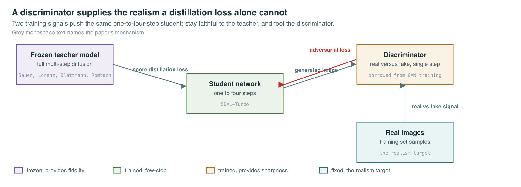
Adversarial diffusion distillation: borrowing the GAN’s realism at one step. Consistency-style distillation still trains the student to match the teacher’s predictions; it does not directly optimize for what a human viewer perceives as sharp, realistic detail, and single-step samples from consistency-style students tend to look softer than multi-step diffusion output. Axel Sauer, Dominik Lorenz, Andreas Blattmann, and Robin Rombach’s adversarial diffusion distillation (ADD) combined two training signals rather than one: a score-distillation loss that keeps the student’s output attached to a frozen teacher diffusion model, and an adversarial loss — a discriminator, borrowed from the GAN training playbook of Chapter 4, whose only job is to tell real images apart from the student’s single-step output (Sauer et al., 2023). The discriminator supplies the missing realism signal that a pure distillation loss cannot; the frozen teacher keeps the student’s output faithful to the prompt and to the base model’s overall composition, preventing the mode collapse that plagued earlier GAN-only text-to-image efforts (Chapter 6, Chapter 7). ADD is the mechanism behind SDXL-Turbo, released the same month, which the paper reports outperforms existing few-step methods — including GANs and LCM — at a single step, and reaches image quality comparable to the full 50-step SDXL base model (Chapter 13) at four steps.

The Mathematics

Progressive distillation reparameterizes the network to predict a quantity the paper calls $v$, a combination of the noise and the clean image, rather than predicting noise directly:

$$v \equiv \alpha_t\,\epsilon - \sigma_t\, x, \qquad \hat x = \alpha_t z_t - \sigma_t\, \hat v_\theta(z_t)$$

Symbol	Meaning
$v$	the network’s training target, a signal/noise combination
$\alpha_t, \sigma_t$	signal- and noise-retention terms at step $t$
$\epsilon, x$	true noise and clean image
$z_t$	noisy latent at step $t$
$\hat v_\theta, \hat x$	network’s predicted $v$, and the clean-image estimate recovered from it

The student’s distillation target $\tilde x$ is the clean-image estimate implied by running the frozen teacher’s DDIM step (Chapter 9) twice in a row; the student is then trained to reach that same target in a single step, with a loss weighted to stay informative even where the signal-to-noise ratio collapses:

$$\mathcal{L}_\theta = w(\lambda_t)\, \big\| \tilde x - \hat x_\theta(z_t) \big\|_2^2, \qquad w(\lambda_t) = \max\!\left(\frac{\alpha_t^2}{\sigma_t^2},\, 1\right)$$

Consistency models parameterize the network so it always outputs an estimate of the clean image, with a built-in identity condition at the boundary of the noising schedule:

$$f_\theta(x, t) = c_{\mathrm{skip}}(t)\, x + c_{\mathrm{out}}(t)\, F_\theta(x, t), \qquad f_\theta(x_\epsilon, \epsilon) = x_\epsilon$$

Symbol	Meaning
$f_\theta$	the consistency function the network computes
$x, t$	noisy input and its timestep
$c_{\mathrm{skip}}(t), c_{\mathrm{out}}(t)$	learned schedule functions controlling the skip connection
$F_\theta$	the raw network before the skip-connection parameterization
$x_\epsilon, \epsilon$	input and timestep at the boundary, nearest to clean data

The property that gives the model its name — self-consistency — requires the network to agree with itself at every point along a shared probability flow ODE trajectory:

$$f_\theta(x_t, t) = f_\theta(x_{t'}, t') \quad \text{for all } t, t' \in [\epsilon, T] \text{ on the same trajectory}$$

Training a consistency model by distillation compares the network’s output at one point on a trajectory to its own (slowly updated) output one step closer to data, where that nearby point is estimated using a single step of a frozen teacher’s ODE solver:

$$\mathcal{L}_{\mathrm{CD}}^N(\theta, \theta^-; \phi) = \mathbb{E}\Big[\lambda(t_n)\, d\big(f_\theta(x_{t_{n+1}}, t_{n+1}),\ f_{\theta^-}(\hat x_{t_n}^\phi, t_n)\big)\Big], \qquad \hat x_{t_n}^\phi := x_{t_{n+1}} + (t_n - t_{n+1})\,\Phi(x_{t_{n+1}}, t_{n+1}; \phi)$$

Symbol	Meaning
$\theta, \theta^-$	student weights, and their exponential moving average used as the training target
$\phi$	frozen teacher diffusion model’s parameters
$\Phi$	one step of an ODE solver using the teacher, advancing $t_{n+1} \to t_n$
$\hat x_{t_n}^\phi$	the nearby target point produced by that one teacher step
$d(\cdot,\cdot)$	distance metric between student and target outputs
$\lambda(t_n)$	per-timestep loss weight

Latent consistency distillation extends this same loss into Stable Diffusion’s latent space, adding the classifier-free guidance scale $\omega$ and text condition $c$ as explicit inputs, and letting the teacher step skip $k$ timesteps at once instead of one:

$$\hat z_{t_n}^{\Psi,\omega} \leftarrow z_{t_{n+k}} + (1+\omega)\,\Psi(z_{t_{n+k}}, t_{n+k}, t_n, c) - \omega\,\Psi(z_{t_{n+k}}, t_{n+k}, t_n, \varnothing)$$

Adversarial diffusion distillation trains the student on a weighted sum of the score-distillation loss above and an adversarial loss from a discriminator:

$$\mathcal{L}(\theta) = \mathcal{L}_{\mathrm{adv}}^G(\theta; \phi) + \lambda\, \mathcal{L}_{\mathrm{distill}}(\theta; \psi)$$

Symbol	Meaning
$\mathcal{L}_{\mathrm{adv}}^G$	student’s adversarial loss against the discriminator
$\mathcal{L}_{\mathrm{distill}}$	score-distillation loss against the frozen teacher
$\theta, \phi, \psi$	student, discriminator, and teacher parameters
$\lambda$	weight balancing the two loss terms, set to 2.5

What It Enabled

None of these four methods retired the others; each trades a different combination of training cost, step count, and image fidelity, and product teams choose among them rather than picking a single winner.

Method	Year	Steps	Training mechanism	Reported result
Progressive distillation	2022	as few as 4	iterative halving, teacher-to-student, no GAN	FID 3.0 on CIFAR-10 at 4 steps; distillation cost comparable to one training run
Consistency models	2023	1 (or 2–3 for a quality bump)	distillation from a pretrained model, or standalone training from scratch	FID 3.55 (CIFAR-10) and 6.20 (ImageNet 64×64) at 1 step
Latent Consistency Models (LCM)	2023	2–4	consistency distillation in latent space, guidance folded into the trajectory	FID 13.53 at 4 steps on LAION-Aesthetic-6.5+, 768×768, built in ~32 A100 GPU-hours
Adversarial Diffusion Distillation (SDXL-Turbo)	2023	1–4	score distillation plus an adversarial loss	outperforms LCM and GANs at 1 step; matches 50-step SDXL quality at 4 steps

The immediate product effect was that “generate an image” stopped requiring a multi-second wait. SDXL-Turbo’s model card explicitly disables classifier-free guidance and negative prompts at inference — the guidance behavior is baked into the single-step network itself rather than computed live — which is the same move LCM’s guidance-conditioned distillation made one layer earlier in the lineage. That is what made real-time, interactive diffusion products possible: a canvas that regenerates as a user drags a slider, or a live camera filter, needs frame-rate latency, not “seconds per image,” and few-step distillation is the specific research thread that closed that gap.

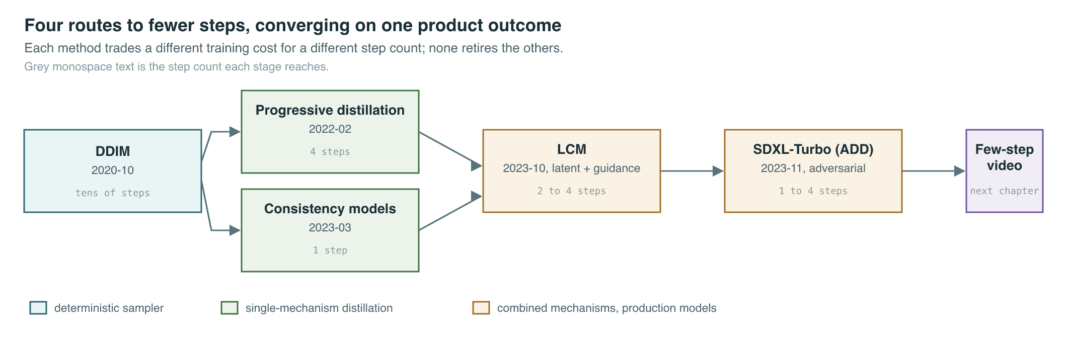
The lineage also runs sideways into other media and into other compression axes. Consistency-style step distillation is the same underlying idea video diffusion models later adopted to make per-clip generation affordable, covered in Video Generation, Chapter 14 rather than re-derived there. And step distillation is a deliberately different compression axis from parameter distillation — shrinking a network’s weight count rather than its sampling schedule — the general teacher-student framing for which, including soft targets and temperature, is covered in Engine Room, Chapter 16; a model can be shrunk both ways at once, and production pipelines increasingly do. Separately, the probability-flow-ODE view that consistency models build on is one of two roads out of DDIM’s deterministic sampler — the other leads to training generative paths as straight lines from the start rather than distilling curved ones after the fact, covered in Chapter 19.

Key Papers

Paper	Authors	Year	Link	Why it matters
Progressive Distillation for Fast Sampling of Diffusion Models	Salimans and Ho	2022	arXiv:2202.00512	First to train step-count down directly, halving a teacher’s steps repeatedly; introduced the $v$-parameterization for stability at few steps
Consistency Models	Song, Dhariwal, Chen, and Sutskever	2023	arXiv:2303.01469	Trained a single network to map any point on a diffusion trajectory directly to its endpoint, enabling true one-step sampling with an optional multi-step quality trade-off
Latent Consistency Models: Synthesizing High-Resolution Images with Few-Step Inference	Luo, Tan, Huang, Li, and Zhao	2023	arXiv:2310.04378	Brought consistency distillation into Stable Diffusion’s guided, text-conditioned latent space, folding classifier-free guidance into the trajectory itself
Adversarial Diffusion Distillation	Sauer, Lorenz, Blattmann, and Rombach	2023	arXiv:2311.17042	Combined score distillation with an adversarial loss to reach single-step, real-time image synthesis at foundation-model quality; the mechanism behind SDXL-Turbo

PM Lens