CLIP: Bridging Text and Image

It is January 2021. OpenAI publishes a visual classifier that never learned a fixed list of categories at all — a quieter release than the text-to-image model the same lab would put out a month later. Within eighteen months this quieter one turns out to matter more — not because it draws anything, but because it hands every later generative model a shared coordinate system in which a sentence and a photograph can be compared directly, as two points in the same space.

Where We Were

Image classifiers built through the 2010s shared a structural assumption: somewhere at training time, a human had fixed a finite list of categories, and the network’s final layer had exactly that many output slots. ImageNet, the dataset released in 2009 that anchored a decade of progress in visual recognition (The Hardware Lottery), defines 1,000 such categories, each backed by roughly a thousand hand-labeled example photographs. A model trained on it is, by construction, an expert on those 1,000 nouns and nothing else. Teaching it a 1,001st category — a new product, a new species, a slang term for an object — means collecting fresh labeled images and retraining or at least fine-tuning the classification head. The taxonomy is not something the model can be handed at inference time; it is baked into the architecture at training time.

Text-conditioned image generation had already found this assumption too rigid to keep, from the opposite direction. StackGAN and AttnGAN (First Words to Pictures) conditioned a generator on a caption rather than a class label, which meant, in principle, an open-ended set of prompts rather than a fixed list. But the text representation those models learned was a byproduct of training one specific generator on one specific dataset of paired captions and photographs — a few tens of thousands of examples, in the case of the bird and flower datasets those papers used. The resulting text embedding space existed to serve that one generator; it was not built, or evaluated, as a general-purpose representation that any other model could reuse, and there was no reason to expect it would transfer to a different generator, a different dataset, or a classification task at all.

Both problems traced back to the same scarce resource: labeled, task-specific data. Building a bigger and more diverse category list, or a richer caption-conditioning space, meant paying for more human annotation. Meanwhile a different resource sat unused at a much larger scale. Hundreds of millions of images on the public internet already came with naturally occurring text attached — captions, alt-text, surrounding article copy — written by people for other people, not for machine-learning pipelines. That text was noisy, informal, and often only loosely related to the image it sat beside. For most of the 2010s, the field treated it as exactly that: noise, unusable for supervised training, worth discarding rather than modeling.

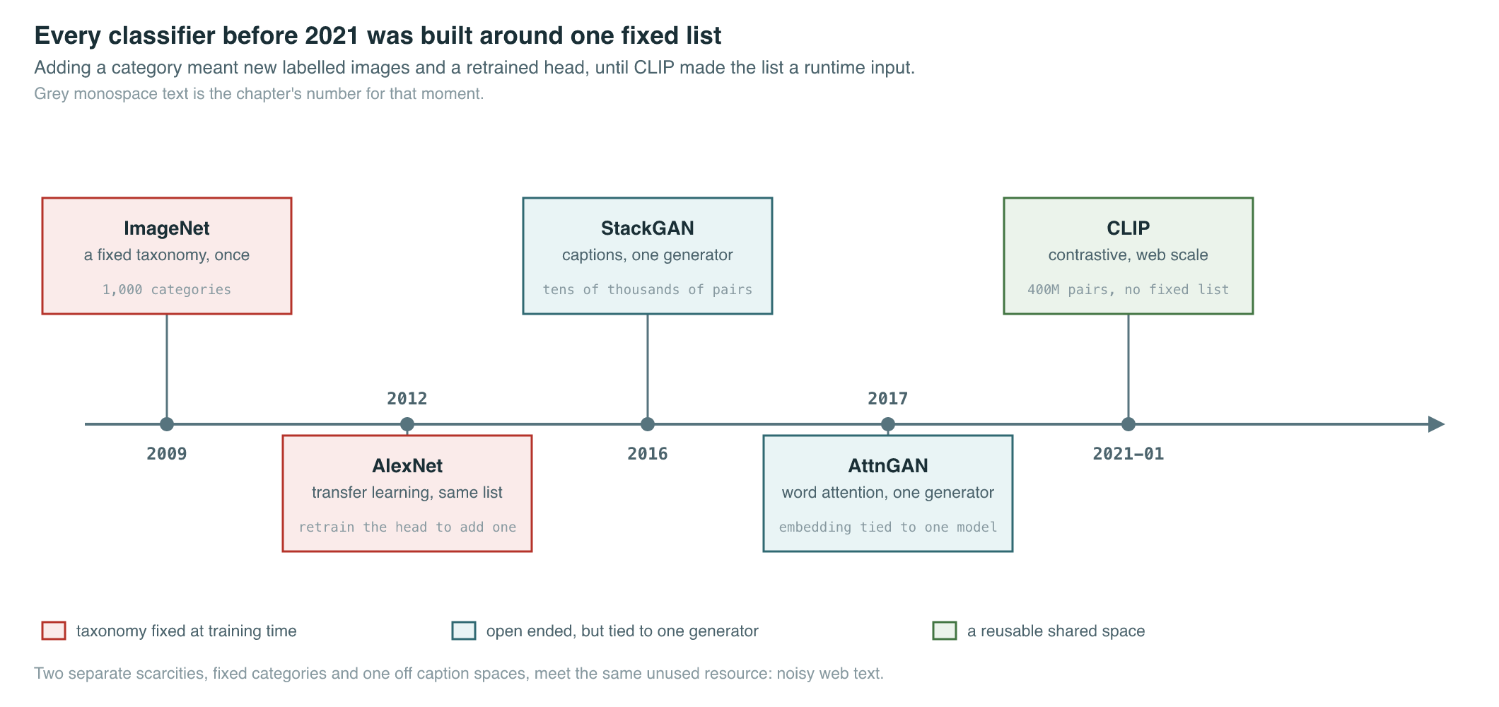
Two different scarcities, a fixed category list and a caption space built for one model, both trace back to the same unused resource: noisy text already sitting next to images on the web. PNG ↓

The open question by the end of 2020 was whether that discarded text was actually a training signal in disguise — whether, at sufficient scale, “loosely related” was good enough, if the objective asked the right question of the data rather than the wrong one.

The Breakthrough

CLIP (Radford et al., 2021) — Contrastive Language-Image Pre-training — answers that question by changing what the network is asked to predict. Instead of classifying an image into one of a fixed set of categories, CLIP trains two separate encoders, one for images and one for text, and asks a purely relative question: given a batch of images and a batch of captions, which caption goes with which image? The image encoder (the paper tests a range of architectures, from an ordinary ResNet-50 up through RN50x64, a ResNet scaled to roughly $64\times$ the compute of ResNet-50 by increasing width, depth, and resolution together, plus several Vision Transformer sizes, with a ViT-L/14 run at 336-pixel resolution performing best) and the text encoder (a Transformer) never see a category label. They only ever see matched and mismatched pairs.

The training data, a set the paper calls WIT (WebImageText), consists of 400 million (image, text) pairs gathered from the public internet — built by searching for images paired with any of 500,000 phrases derived from Wikipedia, which kept the collection topically broad without requiring a single human to inspect or label an individual pair. No annotator ever confirmed that a given photo truly matched its caption; the training objective was designed to tolerate that noise rather than depend on its absence.

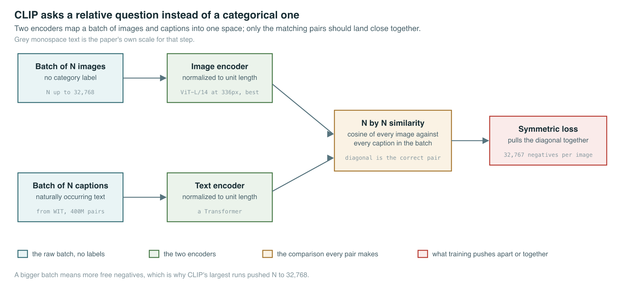
No category ever appears. The only question the network answers is which caption belongs with which image, at whatever scale the batch allows. PNG ↓

Within a training batch of $N$ images and $N$ captions, only the $N$ pairs on the diagonal of the similarity matrix are correct; the remaining $N^2 - N$ off-diagonal combinations are treated as negatives the model must push apart. CLIP’s largest training runs used a batch size of 32,768 — meaning every single image saw 32,767 candidate wrong captions in the same step it saw its one right one, a scale of negative sampling far beyond anything a fixed-category classifier’s cross-entropy loss provides. The paper’s two largest models were correspondingly expensive to train: the wide ResNet variant, RN50x64, took 18 days on 592 V100 GPUs, and the best-performing ViT-L/14 took 12 days on 256 V100 GPUs.

The payoff of this setup shows up at test time, not just in the training loss. Because the text encoder can embed any string, a user can hand CLIP an entirely new classification task — a fresh list of category names it never saw during training — by writing each candidate label into a template such as “a photo of a {label},” embedding all of them, and picking whichever text embedding is closest, by cosine similarity, to the image’s embedding. Nothing is retrained; the classification head is replaced by a lookup in a shared embedding space. The paper reports that this zero-shot approach, ensembled over 80 hand-written prompt templates rather than a single fixed phrase, measurably improves accuracy over the naive single-template version — the ViT-B/16 model’s zero-shot ImageNet accuracy rose from 66.92% with the single template “a photo of a {label}” to 68.57% with the full 80-template ensemble. The best model overall, ViT-L/14 at 336-pixel resolution, reached 76.2% zero-shot top-1 accuracy on ImageNet — matching the accuracy of the original supervised ResNet-50 without training on any of ImageNet’s 1.28 million labeled images. CLIP’s authors also reported that this zero-shot approach was substantially more robust to natural distribution shift than a conventionally trained ImageNet classifier, narrowing the gap between in-distribution and out-of-distribution accuracy by up to 75% relative to a standard ResNet-101.

About five weeks after CLIP’s public announcement, a team at Google pushed the same idea in the opposite direction on the data side. ALIGN (Jia et al., 2021) — submitted to arXiv on February 11, 2021 — asked what happens if the curation step is removed almost entirely rather than tightened. Where CLIP’s WIT dataset was built by querying for pairs matching half a million Wikipedia-derived phrases, ALIGN trained on 1.8 billion image and alt-text pairs scraped directly from web pages with only minimal frequency-based filtering — an order of magnitude more data, an order of magnitude less curation. Its architecture pairs an EfficientNet-L2 image encoder with a BERT-Large text encoder, trained with an effective batch size of 16,384 across 1,024 Cloud TPUv3 cores, on the same contrastive objective CLIP uses. Despite — or, the paper argues, partly because of — skipping the curation step, ALIGN reached 76.4% zero-shot top-1 accuracy on ImageNet, matching CLIP almost exactly, and it clearly outperformed CLIP on cross-modal retrieval, the task of finding the matching caption for an image or the matching image for a caption. The result generalized the lesson CLIP had already suggested: at sufficient scale, noisy, uncurated, naturally occurring text is not a poor substitute for labeled data — it can be trained on directly, and simply pouring in more of it compensates for the noise.

The Mathematics

Notation follows Radford et al. (2021). Let $x_i$ denote the $i$ -th image in a training batch and $y_i$ its paired caption, for $i = 1, \dots, N$ . An image encoder $f$ and a text encoder $g$ map each into a shared embedding space, and both embeddings are normalized to unit length before anything is compared:

\hat{I}_i = \frac{f(x_i)}{\lVert f(x_i) \rVert_2}, \qquad \hat{T}_i = \frac{g(y_i)}{\lVert g(y_i) \rVert_2}

Symbol	Meaning
$x_i, y_i$	the $i$ -th image and its paired caption in the training batch
$f, g$	the image encoder and the text encoder
$\hat{I}_i, \hat{T}_i$	unit-normalized image and text embeddings
$\lVert \cdot \rVert_2$	the Euclidean norm, used to rescale each embedding to unit length

Comparing every image in a batch against every caption in the batch produces an $N \times N$ matrix of scaled similarities:

L_{i,j} = \tau \cdot \hat{I}_i^{\top} \hat{T}_j

Symbol	Meaning
$\tau$	a learned temperature scaling the similarity scores
$L_{i,j}$	the scaled similarity between image $i$ and caption $j$

Training treats this matrix as two interleaved classification problems — for every image, which of the $N$ captions in the batch is the right one, and for every caption, which of the $N$ images is the right one — and minimizes their average as a single symmetric loss:

\mathcal{L} = \frac{1}{2N}\sum_{i=1}^{N}\left[-\log\frac{\exp(L_{i,i})}{\displaystyle\sum_{j=1}^{N}\exp(L_{i,j})} \;-\; \log\frac{\exp(L_{i,i})}{\displaystyle\sum_{j=1}^{N}\exp(L_{j,i})}\right]

$L_{i,i}$ , the diagonal entry, is the similarity between an image and its own correct caption; every other entry in row $i$ or column $i$ is a mismatched pair the model must rate lower. The first term inside the brackets is an ordinary softmax cross-entropy loss: treat image $i$ ‘s row of similarities to all $N$ captions as logits over $N$ classes, and push probability mass onto the correct class $i$ . The second term does the same thing in the other direction, treating caption $i$ ‘s column of similarities to all $N$ images as logits over $N$ image classes. Averaging both directions and over the whole batch is what makes the loss symmetric: the model is penalized equally for a caption failing to identify its image and for an image failing to identify its caption. This is a batch-scale generalization of noise-contrastive estimation — every wrong pairing in the batch is a free negative example, so a larger batch size directly means a harder, more informative training signal, which is why CLIP’s largest runs pushed batch size to 32,768.

Symbol	Meaning
$N$	the number of image-caption pairs in a training batch
$L_{i,i}$	the similarity between a correctly paired image and caption
$\sum_j \exp(L_{i,j})$	normalizing sum over all captions, for the image-to-text direction
$\sum_j \exp(L_{j,i})$	normalizing sum over all images, for the text-to-image direction
$\mathcal{L}$	the final training loss, averaged over both directions and the batch

Once trained, classifying a new image into any list of $K$ candidate categories no longer requires a classification head at all — only a comparison against $K$ text embeddings built from that list:

\hat{y} = \operatorname*{arg\,max}_{k \in \{1,\dots,K\}} \ \hat{I}^{\top} \hat{T}_k

Symbol	Meaning
$\hat{y}$	the predicted class for a new image
$K$	the number of candidate labels supplied at inference time
$\hat{T}_k$	the text embedding of the $k$ -th candidate label’s prompt
$\hat{I}$	the embedding of the new image being classified

What It Enabled

The immediate, measurable consequence was that a classifier’s vocabulary became a runtime input rather than an architectural decision. The comparison below lines up the fixed-taxonomy regime CLIP and ALIGN replaced against what the contrastive approach delivered.

	Fixed-taxonomy classifier (pre-2021)	Contrastive image-text model (CLIP, ALIGN)
Category list	fixed at training time, requires labeled examples per class	supplied at inference time, as arbitrary text
Adding a new category	requires new labeled data and retraining the head	requires writing a new prompt string
Training data	human-labeled datasets (ImageNet: ~1.28M labeled images)	naturally occurring web image-text pairs (CLIP: 400M; ALIGN: 1.8B)
Cross-model reuse	representation tied to the classifier it was trained for	shared embedding space reusable by unrelated downstream models
Zero-shot ImageNet top-1	not applicable (no zero-shot mechanism)	CLIP 76.2%; ALIGN 76.4%

CLIP and ALIGN also make a direct comparison against each other, since both were trained on the same task with very different data strategies:

Metric	CLIP (ViT-L/14, 400M curated pairs)	ALIGN (EfficientNet-L2 + BERT, 1.8B noisy pairs)
Effective batch size	32,768	16,384
Zero-shot ImageNet top-1	76.2%	76.4%
Flickr30K R@1, image-to-text	88.0%	88.6%
Flickr30K R@1, text-to-image	68.7%	75.7%
MSCOCO R@1, image-to-text	58.4%	58.6%
MSCOCO R@1, text-to-image	37.8%	45.6%

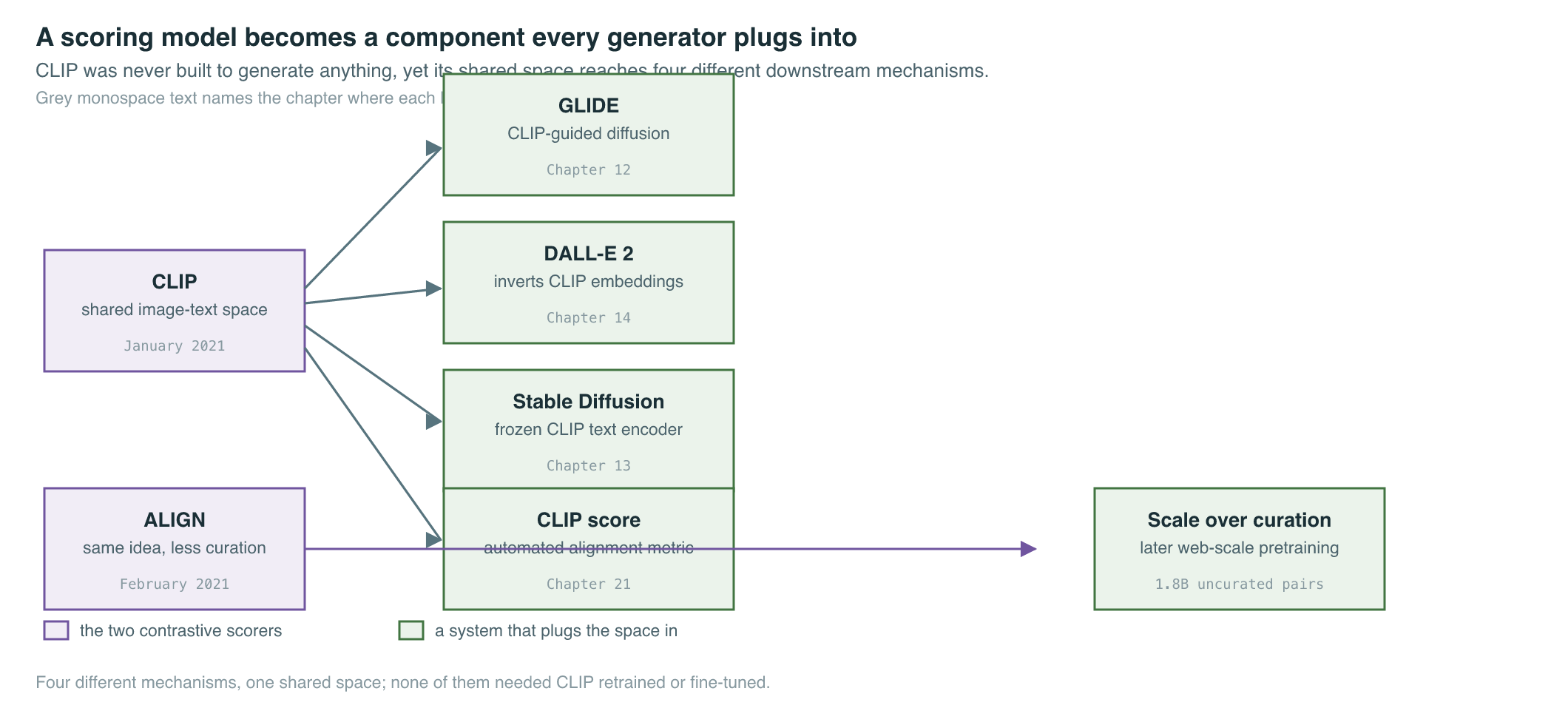
The larger consequence was architectural rather than purely numerical: CLIP’s shared embedding space became a component other generative models could plug into rather than a classifier’s endpoint. Within the same year, GLIDE steered a text-conditioned diffusion model’s sampling process using gradients of similarity in a CLIP-like joint space, a technique this book covers alongside its autoregressive counterpart in DALL-E and GLIDE. The following year, DALL-E 2 built an entire generation pipeline around inverting CLIP’s image embedding back into a picture, an architecture covered in The Year Images Went Mainstream. Stable Diffusion’s original release used a frozen CLIP ViT-L/14 text encoder as its default conditioning signal, folding CLIP directly into the latent diffusion pipeline described in Latent Diffusion and Stable Diffusion. And because CLIP gives any image-caption pair a single similarity number without a human rater, cosine similarity in CLIP’s embedding space became a standard automated stand-in for “does this generated image match this prompt,” a metric this book returns to in Evaluation, Provenance, and Safety.

CLIP was built to score, not to draw. Every arrow on the right is a later model reusing that score for a job its authors never built it for. PNG ↓

Key Papers

Paper	Authors	Year	Link	Why it matters
Learning Transferable Visual Models From Natural Language Supervision	Radford, Kim, Hallacy, Ramesh, Goh, Agarwal, Sastry, Askell, Mishkin, Clark, Krueger, Sutskever	2021	arXiv:2103.00020	Introduced CLIP: contrastive pretraining on 400M web image-text pairs, 76.2% zero-shot ImageNet top-1, and the shared embedding space every later text-to-image model builds on
Scaling Up Visual and Vision-Language Representation Learning With Noisy Text Supervision	Jia, Yang, Xia, Chen, Parekh, Pham, Le, Sung, Li, Duerig	2021	arXiv:2102.05918	Showed the same contrastive recipe scales to 1.8B uncurated pairs, matching CLIP’s zero-shot accuracy and beating it on retrieval, proving scale can substitute for curation

PM Lens

The habit this chapter left me with is asking, before greenlighting any “search your photos by description” or “tag this image automatically” feature, whether the team actually needs a fine-tuned classifier or just a CLIP checkpoint and a prompt string. Because OpenAI released CLIP’s weights openly, most of that category of feature is a local embedding lookup against a vector database, not a metered inference API call — the cost structure looks nothing like paying per token for an LLM, and product teams that price it as if it does are usually overbuilding. The other number I keep in view is the 76.2%-versus-76.4% split between CLIP and ALIGN: two teams, two very different data strategies — one curated and modest, one enormous and unfiltered — landed on essentially the same zero-shot accuracy. When someone pitches “our advantage is a cleaner dataset,” this chapter is why I ask what scale of uncurated data would erase that advantage instead, before treating curation as a permanent moat.

Search