Taming GAN Training

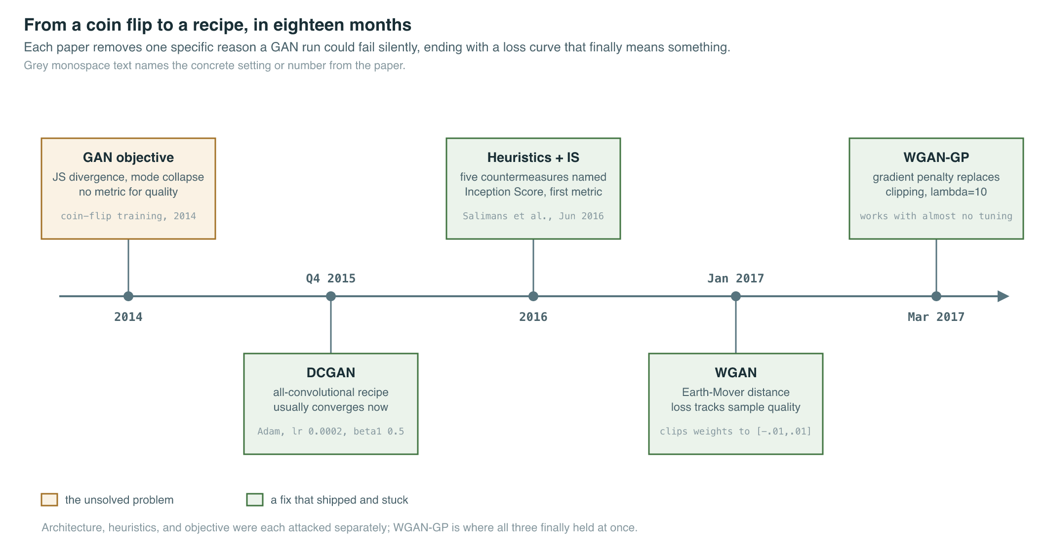
It is late 2015. The adversarial objective works in principle — a generator and a discriminator playing a minimax game can, in theory, converge to a generator that samples from the true data distribution — but in practice GAN training is a coin flip. Runs diverge, generators collapse onto a handful of outputs, and the only diagnostic tool is staring at a grid of samples every few thousand steps. Over the following eighteen months, three papers turn that coin flip into a recipe: one fixes the architecture, one catalogs the failure modes and gives them names, and two rewrite the objective itself so that a single number — the loss — finally tells you whether training is working.

Where We Were

The original GAN formulation, Goodfellow et al.’s 2014 minimax game between a generator and a discriminator, its Jensen-Shannon-divergence interpretation, and the mode-collapse failure mode it invites, is taught in full in Chapter 3. This chapter starts from that objective as a given and asks a narrower question: given that the game is sound in theory, why is it so hard to run in practice, and what changed between 2014 and 2017 to make it tractable?

By late 2015, three practical problems dominated any attempt to train a GAN at scale beyond small, fully-connected toy networks. First, there was no reliable architectural recipe: convolutional generators and discriminators, the natural choice for images, were notoriously prone to diverge, and early attempts to stack standard convolutional-network components — pooling layers, fully connected heads — into an adversarial pair mostly failed. Second, the training dynamic itself was fragile in ways the 2014 paper had only partially anticipated: if the discriminator got too good too fast, its gradient with respect to the generator’s parameters vanished, and the generator stopped learning; if the generator found one output that reliably fooled the discriminator, it had no incentive to produce anything else, and training collapsed onto a handful of modes. Third, and perhaps most consequential for the field’s pace of progress, there was no quantitative way to answer “is this run any good?” without a human looking at generated images. Two different training runs could report similar discriminator and generator losses while producing wildly different sample quality, because the GAN loss does not correlate with sample fidelity the way, say, cross-entropy loss correlates with classification accuracy.

Architecture, heuristics, and objective were each attacked separately; WGAN-GP is where all three finally held at once. PNG ↓

That third problem — no metric — is what made the other two so hard to fix by trial and error. Without a number that tracked quality, every architectural or hyperparameter change had to be evaluated by eye, across enough random seeds to separate signal from the training procedure’s inherent instability. The three papers anchoring this chapter attack the problem from both ends: architecture and heuristics first, then the mathematics of the objective itself.

The Breakthrough

Deep Convolutional GANs (Radford et al., 2015), submitted to arXiv in November 2015, did not change the adversarial objective at all. Its contribution was empirical: a specific set of architectural constraints that, applied together, took convolutional GAN training from “usually diverges” to “usually converges.” The paper’s guidelines were concrete enough to be copied wholesale: replace every pooling layer with a strided convolution in the discriminator and a fractionally-strided (transposed) convolution in the generator; remove fully connected hidden layers entirely, so the network is all-convolutional; use batch normalization in both networks, except at the generator’s output layer and the discriminator’s input layer; use ReLU activations in the generator everywhere except the output layer, which uses Tanh; and use LeakyReLU, with the leak slope set to 0.2, in the discriminator at every layer.

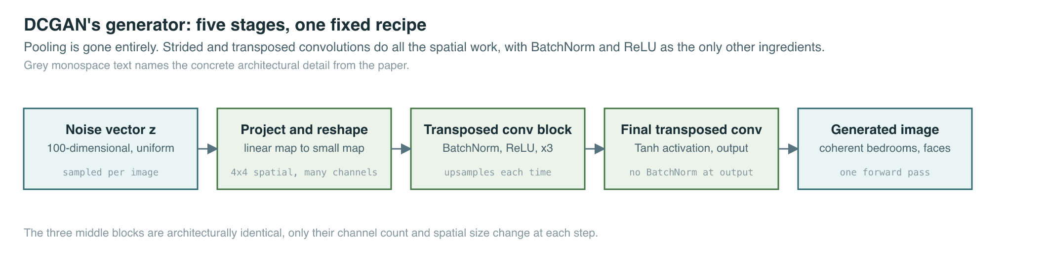
The three middle blocks are architecturally identical, only their channel count and spatial size change at each step. PNG ↓

Two training details mattered as much as the architecture. DCGAN used the Adam optimizer with a learning rate of 0.0002, well below Adam’s suggested default of 0.001, and reduced Adam’s first-moment decay term, $\beta_1$ , from its default 0.9 to 0.5 — a small change the authors found necessary to stabilize training. Mini-batches of 128 images, weights initialized from a zero-centered Normal distribution with standard deviation 0.02, and no other tricks. The result was a generator that reliably produced coherent bedroom scenes and faces, and whose learned latent space supported vector arithmetic on semantic attributes — evidence that the network had learned a structured representation, not memorized training examples.

DCGAN fixed the architecture, but it did not fix the underlying instability of the adversarial game — it made instability more manageable, not absent. Improved Techniques for Training GANs (Salimans et al., 2016), submitted in June 2016 by a team including the original GAN paper’s lead author, catalogued the remaining failure modes and proposed five concrete countermeasures. Feature matching redirects the generator’s objective away from directly maximizing the discriminator’s output and toward matching the discriminator’s intermediate-layer statistics on real versus generated data, a softer target that is harder for the generator to game with a single degenerate output. Minibatch discrimination lets the discriminator look at multiple samples at once so it can directly penalize the generator for producing outputs that are too similar to each other, attacking mode collapse where it happens — across a batch, not within a single image. Historical averaging adds a penalty term based on each player’s distance from the running average of its own past parameters, an idea borrowed from fictitious-play algorithms in game theory. One-sided label smoothing softens only the “real” target — from 1 to a value like 0.9 — leaving the “fake” target at 0, which avoids a specific failure mode where a smoothed fake target actively teaches the discriminator to send bad gradients on regions of input space it has never seen. Virtual batch normalization normalizes each example using statistics from a fixed reference batch chosen once at the start of training, plus its own statistics, removing batch normalization’s dependence on which other examples happen to share the current minibatch.

The same paper also introduced the field’s first widely adopted automatic quality metric, the Inception Score — a way to put a number on sample quality without a human in the loop, discussed in the Mathematics section below.

None of this addressed the theoretical reason the GAN loss failed to track quality. That took a reframing of the objective itself. Wasserstein GAN (Arjovsky et al., 2017), submitted in January 2017, replaced the Jensen-Shannon divergence at the heart of the original GAN objective with the Earth-Mover (Wasserstein-1) distance, and replaced the discriminator’s job — classifying real versus fake — with a new job: estimating that distance directly. The practical upshot, developed in the Mathematics section, was a training signal that behaved like a real loss function: it tended to decrease as training progressed, and it correlated with the visual quality of generated samples, so a WGAN loss curve could be read at a glance the way a classifier’s cross-entropy loss can be. The paper’s own implementation, however, enforced its key mathematical requirement with weight clipping — after every update, all critic weights were clamped into $[-0.01, 0.01]$ — a constraint the authors themselves flagged as “a terrible way” to enforce it, one prone to either vanishing or exploding critic gradients depending on the clipping threshold and network depth.

Improved Training of Wasserstein GANs (Gulrajani et al., 2017), submitted in March 2017, replaced weight clipping with a gradient penalty: instead of clamping weights, the loss directly penalizes the critic whenever the norm of its gradient, at points interpolated between real and generated samples, strays from 1. WGAN-GP dropped weight clipping’s capacity bottleneck — clipped critics tended toward simple, near-linear functions, because clipping caps how much any single layer’s weights can differentiate inputs — and trained with Adam rather than RMSProp, the optimizer WGAN had recommended specifically because Adam’s momentum interacted badly with weight clipping’s non-stationary loss landscape. The result, reported across a range of architectures with almost no per-model hyperparameter tuning, was the first GAN training recipe that could be dropped onto a new architecture and simply be expected to work.

The Mathematics

The original GAN’s discriminator estimates a probability and the generator is trained against the resulting Jensen-Shannon divergence between the real and generated distributions — mathematics owned by Chapter 3. The Jensen-Shannon divergence has a specific weakness: when two distributions have little or no overlapping support, which is the common case early in training when the generator’s output looks nothing like real data, the divergence saturates at a constant and its gradient vanishes almost everywhere. WGAN’s fix starts from a different notion of distance between distributions, one that stays smooth and informative even when the distributions do not overlap: the Wasserstein-1, or Earth-Mover, distance. Computing it directly is intractable, but the Kantorovich-Rubinstein duality gives an equivalent form that a neural network can approximate:

W(P_r, P_g) = \sup_{\|f\|_L \le 1} \; \mathbb{E}_{x \sim P_r}[f(x)] - \mathbb{E}_{x \sim P_g}[f(x)]

Symbol	Meaning
$W(P_r, P_g)$	Wasserstein-1 distance between the real and generated distributions
$P_r, P_g$	real and generator-induced data distributions
$f$	a scalar-valued function, the candidate “critic”
$\\|f\\|_L \le 1$	the 1-Lipschitz constraint on $f$
$\sup$	supremum — the largest value achievable over all valid $f$
$\mathbb{E}$	expectation, an average over samples drawn from the given distribution

A neural network $f_w$ , parameterized by weights $w$ , stands in for the supremum over all 1-Lipschitz functions, turning the distance estimate into a network trained against the generator in the same adversarial loop as before — except this network, now called the critic rather than the discriminator, outputs an unbounded real number instead of a probability, and there is no sigmoid at its output:

\min_{G} \; \max_{w \,:\, \|f_w\|_L \le 1} \;\; \mathbb{E}_{x \sim P_r}[f_w(x)] - \mathbb{E}_{z \sim p(z)}[f_w(G(z))]

Symbol	Meaning
$G$	the generator network
$w$	the critic’s parameters, constrained so $f_w$ stays 1-Lipschitz
$f_w$	the critic, a neural network standing in for the supremum in the Wasserstein dual
$P_r$	the real data distribution
$z, p(z)$	a noise vector and the simple prior distribution it is drawn from
$G(z)$	the generator’s output given noise $z$

The constraint $\|f_w\|_L \le 1$ has to be enforced somehow, since nothing about an ordinary neural network’s parameterization keeps it 1-Lipschitz on its own. The original WGAN paper’s answer was to clip every weight into a fixed range after each update; WGAN-GP’s answer was a soft penalty on the critic’s gradient norm, added directly to the loss:

\begin{aligned} L &= \mathbb{E}_{\tilde{x} \sim P_g}[D(\tilde{x})] \;-\; \mathbb{E}_{x \sim P_r}[D(x)] \;+\; \lambda \, \mathbb{E}_{\hat{x} \sim P_{\hat{x}}}\Big[\big(\|\nabla_{\hat{x}} D(\hat{x})\|_2 - 1\big)^2\Big] \\ \hat{x} &= \epsilon x + (1-\epsilon)\tilde{x}, \qquad \epsilon \sim U[0,1] \end{aligned}

The first two terms are the same critic objective as before, with $D$ now standing in for the critic and $\tilde{x} = G(z)$ for a generated sample. The third term is new: $\hat{x}$ is a random point on the straight line between a real sample $x$ and a generated sample $\tilde{x}$ , chosen by mixing them with a random weight $\epsilon$ drawn uniformly between 0 and 1, and the penalty pushes the norm of the critic’s gradient at that point, $\|\nabla_{\hat{x}} D(\hat{x})\|_2$ , toward exactly 1 — which is what being 1-Lipschitz requires almost everywhere. $\lambda$ , set to 10 in the paper, weights how strongly this penalty is enforced relative to the critic objective itself. What it buys you: a differentiable constraint that leaves the critic free to use its full representational capacity, instead of weight clipping’s blunt cap on every weight, and one that does not depend on network depth or clipping threshold the way clipped gradients do.

Symbol	Meaning
$L$	the critic’s full training loss, including the penalty
$D$	the critic network (WGAN-GP’s name for $f_w$ )
$x, \tilde{x}$	a real sample and a generated sample
$\hat{x}$	a random interpolation point between $x$ and $\tilde{x}$
$\epsilon$	interpolation weight, drawn from a uniform distribution on $[0,1]$
$\lambda$	gradient penalty coefficient, 10 in the paper
$\nabla_{\hat{x}} D(\hat{x})$	gradient of the critic’s output with respect to its input at $\hat{x}$

WGAN-GP trained the critic five times for every one generator update ( $n_{\text{critic}} = 5$ , carried over from the original WGAN setup) using Adam with learning rate 0.0001, $\beta_1 = 0$ , and $\beta_2 = 0.9$ — a return to Adam, now safe because the gradient penalty, unlike weight clipping, does not create the non-stationary loss landscape that had made Adam’s momentum term misbehave. Adam’s own mechanics, and why $\beta_1$ and $\beta_2$ do what they do, are covered in The Engine Room, Chapter 5; batch normalization’s mechanics are covered in The Engine Room, Chapter 6.

The other piece of mathematics this era introduced was a way to score sample quality without a human, the Inception Score:

\mathrm{IS}(G) = \exp\Big(\mathbb{E}_{x \sim p_g}\big[D_{KL}\big(p(y \mid x) \,\|\, p(y)\big)\big]\Big)

Symbol	Meaning
$\mathrm{IS}(G)$	the Inception Score of generator $G$
$p_g$	the generator’s output distribution
$p(y \mid x)$	the Inception classifier’s label distribution for one generated sample
$p(y)$	the marginal label distribution, averaged over many generated samples
$D_{KL}$	Kullback-Leibler divergence between the two label distributions
$\exp$	exponential, rescaling the score onto a more interpretable range

On CIFAR-10, the paper reported an Inception Score of 8.09 ± 0.07 for its best configuration, against 11.24 ± 0.12 for real CIFAR-10 images themselves — a first quantitative anchor for “how far is a generator from real data,” and the ancestor of the FID metric that would later replace it, covered in Chapter 21.

What It Enabled

Before this chapter’s papers, running a convolutional GAN was closer to alchemy than engineering: an architecture that worked for one dataset might diverge on another, and the only way to know was to watch it train. After them, GAN training had a default architecture, a named list of failure modes with named countermeasures, and — with WGAN-GP — an objective whose loss curve was actually informative.

	Before, GAN circa 2014–2015	After, DCGAN + WGAN-GP recipe, 2017
Architecture guidance	None specific to convolutional nets; frequent divergence	All-convolutional, BatchNorm, ReLU/LeakyReLU, no pooling or FC layers
Loss as a training signal	Uninformative — can look fine while samples degrade	Approximates Wasserstein distance; tracks sample quality
Lipschitz enforcement	Not applicable (no such constraint existed)	Gradient penalty, not weight clipping — full critic capacity retained
Optimizer	Adam, default hyperparameters, frequent instability	Adam, tuned $\beta_1$ (DCGAN) or $\beta_1=0,\beta_2=0.9$ (WGAN-GP)
Quality measurement	Human inspection of sample grids	Inception Score — automatic, if imperfect, quantitative metric
Cross-architecture reliability	Ad hoc; hyperparameters rarely transferred	WGAN-GP reported stable training “with almost no hyperparameter tuning” across varied architectures

The direct consequence was scale. A training recipe that reliably converged and told you when it was working is a precondition for scaling anything up — you cannot productively spend a larger compute budget on a procedure whose failure mode is silent divergence discovered a week later. Progressive growing and the large-batch, large-model GANs that followed — BigGAN, StyleGAN, and StyleGAN2 — inherited this chapter’s stability toolkit directly, and StyleGAN’s own regularization techniques descend from the same gradient-penalty idea applied to the discriminator. That lineage is Chapter 6.

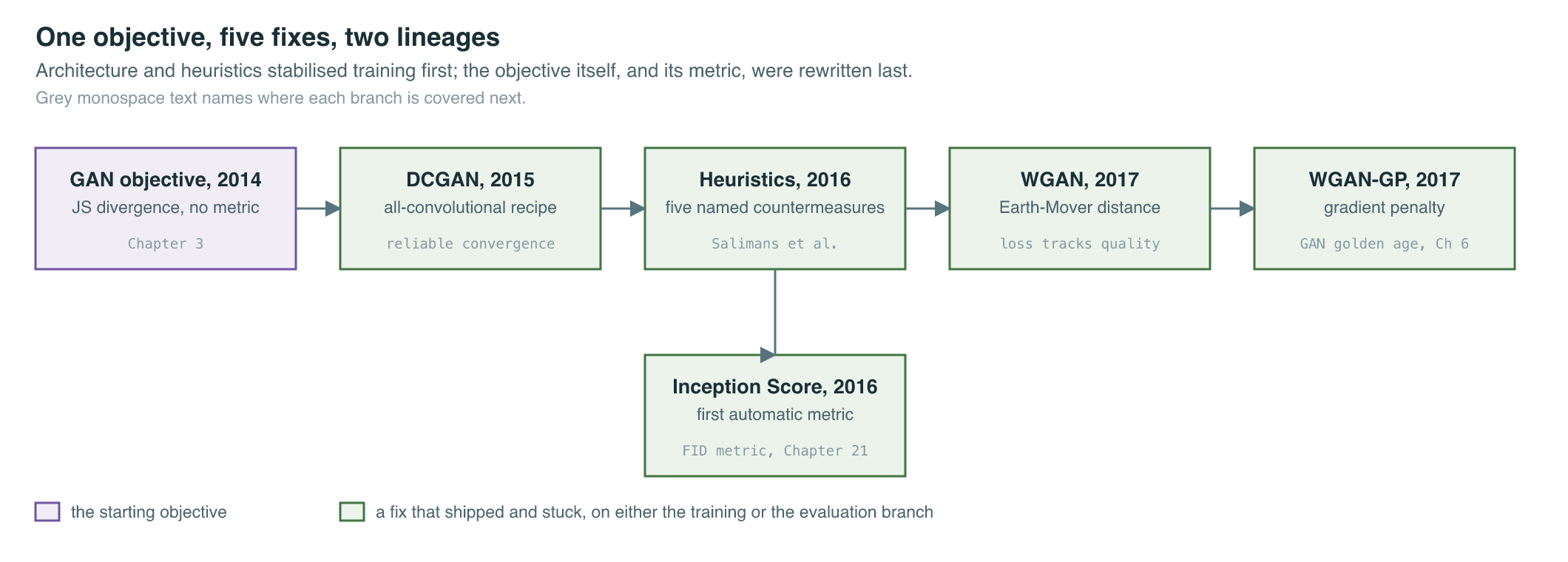
Architecture and heuristics fixed the training branch; the same 2016 paper also opened a separate evaluation branch that runs to Chapter 21. PNG ↓

Evaluation followed the same arc as training. The Inception Score gave the field its first automatic number, but it measured recognizability against an ImageNet-trained classifier’s categories and said nothing about how close a generated distribution actually sat to the real one in feature space — a gap the Fréchet Inception Distance closed a few months later, covered in Chapter 21. And the stability work itself turned out to be adversarial-training-specific rather than generative-modeling-general: when diffusion models arrived a few years later, covered starting in Chapter 8, they sidestepped this entire chapter’s problem by training against a stable regression-style denoising loss with no min-max game at all — the instability GANs spent 2015 to 2017 taming was never a property of image generation itself, only of the adversarial formulation of it.

Key Papers

Paper	Authors	Year	Link	Why it matters
Unsupervised Representation Learning with Deep Convolutional Generative Adversarial Networks	Radford, Metz, and Chintala	2015	arXiv:1511.06434	Gave convolutional GANs a specific, reusable architecture that reliably converged
Improved Techniques for Training GANs	Salimans, Goodfellow, Zaremba, Cheung, Radford, and Chen	2016	arXiv:1606.03498	Named the remaining failure modes, proposed five countermeasures, and introduced the Inception Score
Wasserstein GAN	Arjovsky, Chintala, and Bottou	2017	arXiv:1701.07875	Replaced JS divergence with the Wasserstein distance, making the loss track sample quality
Improved Training of Wasserstein GANs	Gulrajani, Ahmed, Arjovsky, Dumoulin, and Courville	2017	arXiv:1704.00028	Replaced weight clipping with a gradient penalty, the first widely reliable GAN recipe

PM Lens

The lesson from this chapter that I still apply is not about GANs specifically — it is about shipping anything whose failure mode is silent. A GAN whose loss curve looked reasonable could still be collapsed, and the only way to find out was to look at outputs, which is expensive to do continuously and easy to skip under deadline pressure. That is the same trap I see in generative products today: an LLM eval that tracks a proxy metric instead of the thing users actually care about will let a regression through just as quietly. Before I approve a launch metric for any generative feature, I ask the WGAN question — does this number actually move with output quality, or does it just move? DCGAN and WGAN-GP mattered commercially not because they made GANs bigger, but because they made a bad run cheap to detect, which is the actual unlock: compute is a budget line, but undetected failure is the one that burns it without producing anything.

Search