Variational Autoencoders

It is December 2013. Deep networks can classify images better than any previous method, but asking one to imagine a plausible new image — to sample from a model of the data rather than just discriminate it — remains mostly unsolved. A two-author paper posted to arXiv on December 20 shows how to train a directed latent-variable model and its approximate-inference network jointly, by backpropagation, using a trick as simple as adding noise after a multiplication. Within fourteen months the same idea has been rediscovered independently, generalized to deep hierarchies, and extended into a recurrent network that draws images stroke by stroke.

Where We Were

The previous chapter (The Generative Problem) framed the task: learn a model of $p(x)$ that can both score images and sample new ones. By the early 2010s, deep learning had produced excellent discriminative models but the generative side of the field was still leaning on machinery from the 1990s. Directed latent-variable models — a prior over an unobserved code $z$, a likelihood $p(x \mid z)$ generating the observed data — were the natural framework, but they carried a structural cost: for anything but the simplest priors and likelihoods, the true posterior $p(z \mid x)$ is intractable, because computing it requires integrating over every possible $z$.

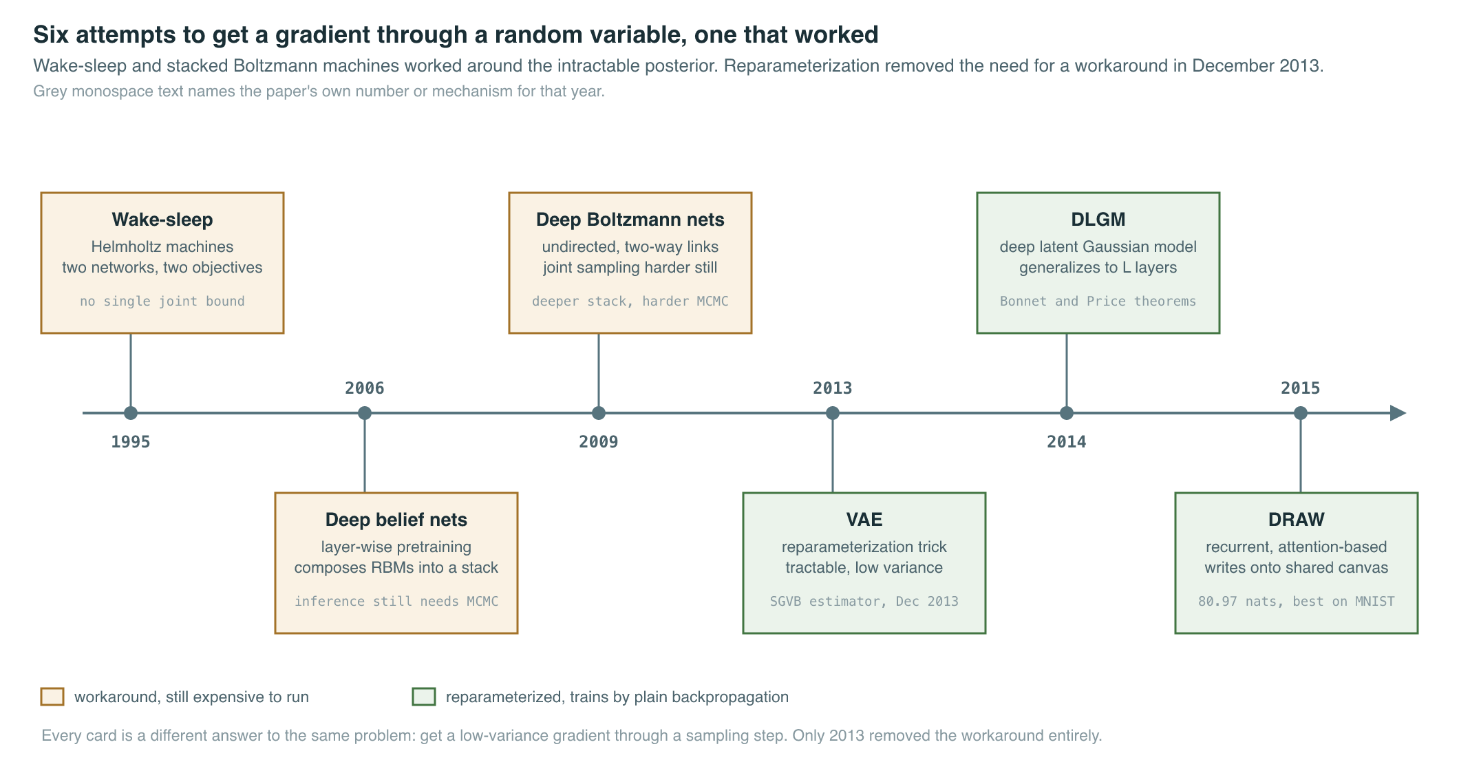
Two families of workaround existed. The wake-sleep algorithm for Helmholtz machines (Hinton, Dayan, Frey & Neal, 1995) trained a recognition network and a generative network in alternating passes, but the two networks optimized different objectives that did not correspond to a single joint bound — an awkward, two-headed compromise. Sampling-based alternatives such as Monte Carlo EM used expensive iterative sampling per datapoint, which scaled poorly to large datasets and did not amortize: every new image required fresh inference work from scratch. Mean-field variational Bayes offered a principled bound but usually demanded closed-form expectations that were themselves intractable for anything built from a multi-layer neural network. Deep belief nets and deep Boltzmann machines (Deep Belief Nets) sidestepped some of this with layer-wise pretraining, but inference in an undirected model brings its own expensive machinery.

The missing piece was a way to train an inference network — a function approximating $p(z \mid x)$ — jointly with the generative model, using plain stochastic gradient descent, with variance low enough to actually converge. The obvious estimator for a gradient through a sampling step, the score-function or REINFORCE-style estimator, has notoriously high variance. The field needed a different way to route gradients through a random variable.

The Breakthrough

Auto-Encoding Variational Bayes (Kingma & Welling, December 2013) supplied the missing piece by changing where the randomness sits, in what the paper calls, plainly, “quite simple” (Kingma & Welling, 2013). Rather than sampling $z$ directly from a distribution parameterized by the network — a step through which gradients cannot flow cleanly — the model samples a fixed noise variable $\epsilon$ from a distribution with no learned parameters, and computes $z$ as a deterministic, differentiable function of $\epsilon$ and the network’s output. This is the reparameterization trick. Because the only source of randomness is now independent of the parameters being optimized, ordinary backpropagation flows through the sampling step, and the resulting gradient estimator — the paper names it the Stochastic Gradient Variational Bayes (SGVB) estimator — has far lower variance than the score-function alternative.

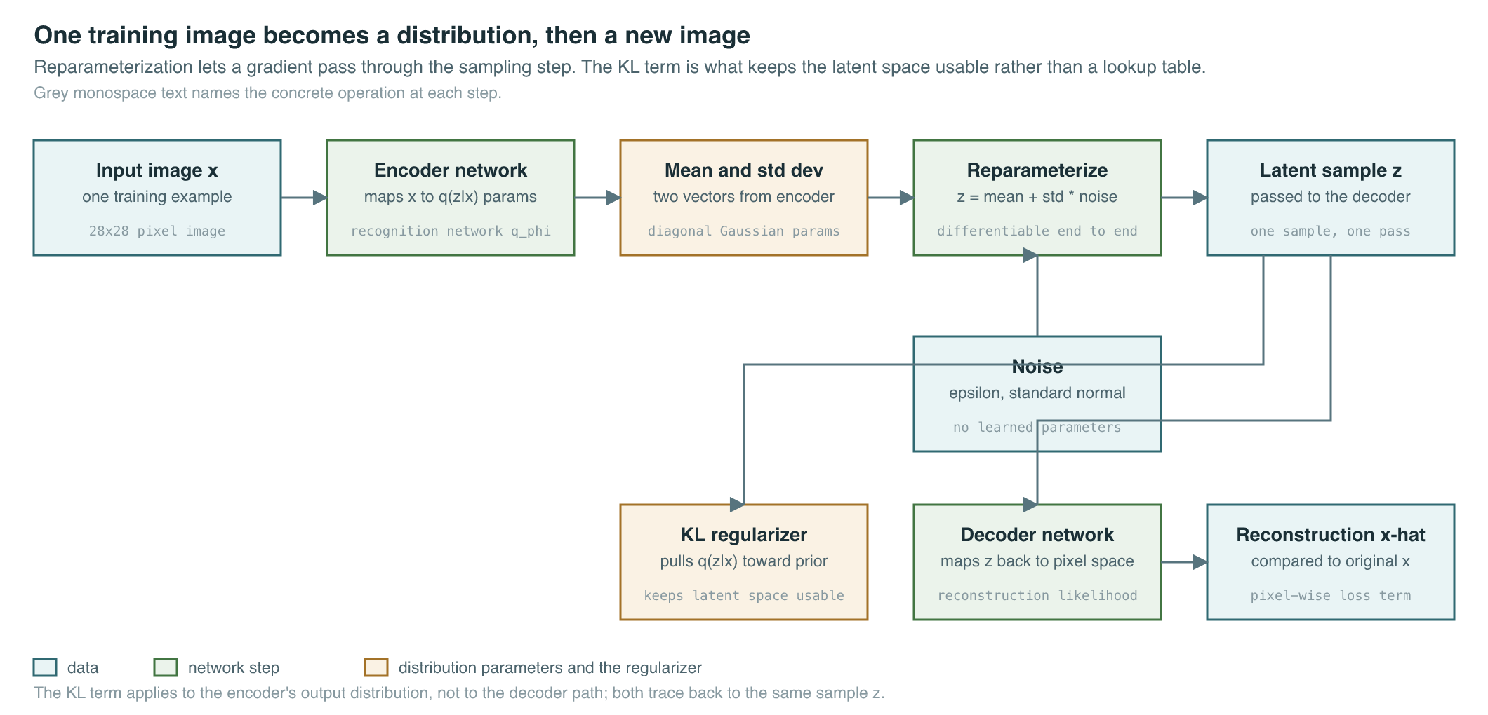
The paper packages this trick into the Auto-Encoding VB (AEVB) algorithm: a neural network (the encoder or recognition model) maps a datapoint $x$ to the parameters of an approximate posterior $q_\phi(z \mid x)$; a sample $z$ is drawn via reparameterization; a second network (the decoder) maps $z$ back to a distribution over $x$. Both networks train jointly by ascending a single objective, the evidence lower bound, computed on random minibatches. When the recognition and generative networks are both neural networks, Kingma and Welling give this construction a new name: the variational auto-encoder.

The design compresses cleanly into an architecture diagram, and the connection to ordinary autoencoders is deliberate: the KL term against the prior is what turns a bottleneck into a generative latent space rather than a mere compression code.

Twenty-seven days later, a second group reached the same destination from a different direction. Stochastic Backpropagation and Approximate Inference in Deep Generative Models (Rezende, Mohamed & Wierstra, January 2014) derived what it calls Gaussian backpropagation from two classical results in probability — Bonnet’s theorem and Price’s theorem — to obtain gradient rules for expectations under a Gaussian, then showed those rules reduce to the same location-scale reparameterization (Rezende et al., 2014). The paper is explicit about the coincidence: “Concurrently with this paper, Kingma & Welling (2014) present an alternative discussion of stochastic backpropagation. Our approaches were developed simultaneously and provide complementary perspectives on the derivation of stochastic backpropagation rules.” Where Kingma and Welling built a two-layer encoder-decoder pair, Rezende, Mohamed and Wierstra generalized immediately to deep latent Gaussian models (DLGMs) — stacks of $L$ layers of Gaussian latent variables, each layer’s activation a nonlinear transform of the layer above it plus Gaussian noise, with an explicit recognition model regularized by injected bit-flip and dropout-style noise at the input to keep it from overfitting to seen data.

Thirteen months after that, DRAW — A Recurrent Neural Network For Image Generation (Gregor, Danihelka, Graves, Rezende & Wierstra, February 2015) — took the same encoder-recognition-decoder pairing and made it iterative (Gregor et al., 2015). Instead of one encode-sample-decode pass per image, DRAW runs a pair of recurrent networks for a fixed number of timesteps: at each step the encoder reads a piece of the target image, updates a latent code, and the decoder writes an update onto a shared canvas that accumulates across steps. The paper frames the motivation directly: a person asked to “recreate a visual scene” does so “in a sequential, iterative fashion,” with “rough outlines… gradually replaced by precise forms” — not in a single shot. DRAW added a second ingredient beyond recurrence — a differentiable spatial attention mechanism built from a grid of two-dimensional Gaussian filters, which lets the network choose, at each timestep, exactly where on the canvas to read from and write to. Because the attention window’s center and zoom are themselves smooth functions of the decoder’s hidden state, the whole system — recurrence, attention, and the underlying VAE machinery — trains end to end with the same reparameterized gradient Kingma, Welling, Rezende, Mohamed and Wierstra had introduced over the preceding fourteen months.

The Mathematics

Notation follows Kingma & Welling (2013): $x$ is an observed datapoint, $z$ is a continuous latent variable, $p_\theta(z)$ and $p_\theta(x \mid z)$ are the generative model’s prior and likelihood with parameters $\theta$, and $q_\phi(z \mid x)$ is the recognition model — the encoder — with parameters $\phi$.

The marginal log-likelihood of a single datapoint decomposes exactly, with no approximation, into two terms:

$$\log p_\theta(x) = D_{KL}\!\left(q_\phi(z \mid x) \,\|\, p_\theta(z \mid x)\right) + \mathcal{L}(\theta, \phi; x)$$

Symbol	Meaning
$x$	an observed datapoint, e.g. one image
$z$	continuous latent variable for that datapoint
$\theta$	parameters of the generative model, decoder
$\phi$	parameters of the recognition model, encoder
$q_\phi(z \mid x)$	approximate posterior produced by the encoder
$p_\theta(z \mid x)$	true posterior — intractable, never computed
$D_{KL}$	Kullback-Leibler divergence between two distributions
$\mathcal{L}(\theta, \phi; x)$	the evidence lower bound, ELBO — what training maximizes

The ELBO itself can be rewritten in a form that separates a regularizer from a reconstruction term:

$$\mathcal{L}(\theta, \phi; x) = -D_{KL}\!\left(q_\phi(z \mid x) \,\|\, p_\theta(z)\right) + \mathbb{E}_{q_\phi(z \mid x)}\!\left[\log p_\theta(x \mid z)\right]$$

Sampling $z$ inside that expectation is exactly the step that ordinary backpropagation cannot pass through. The reparameterization trick rewrites the sample as a deterministic function of noise:

$$z = \mu_\phi(x) + \sigma_\phi(x) \odot \epsilon, \qquad \epsilon \sim \mathcal{N}(0, \mathbf{I})$$

Symbol	Meaning
$z$	the latent sample actually passed to the decoder
$\mu_\phi(x)$	encoder’s output mean, function of $x$ and $\phi$
$\sigma_\phi(x)$	encoder’s output standard deviation
$\epsilon$	auxiliary noise, sampled once per forward pass
$\odot$	elementwise, Hadamard, multiplication

When the prior and posterior are both Gaussian, the KL term integrates in closed form, and Kingma and Welling’s full per-datapoint training objective becomes:

$$\mathcal{L}(\theta, \phi; x^{(i)}) \simeq \frac{1}{2}\sum_{j=1}^{J}\left(1 + \log\big((\sigma_j^{(i)})^2\big) - (\mu_j^{(i)})^2 - (\sigma_j^{(i)})^2\right) + \frac{1}{S}\sum_{s=1}^{S} \log p_\theta\!\left(x^{(i)} \mid z^{(i,s)}\right)$$

Symbol	Meaning
$J$	number of latent dimensions
$\mu_j^{(i)}, \sigma_j^{(i)}$	encoder’s mean and standard deviation, dimension $j$, point $i$
$S$	number of reparameterized samples per datapoint, per gradient step
$z^{(i,s)}$	the $s$-th reparameterized sample for datapoint $i$

DRAW extends this same objective across timesteps rather than deriving a new one. With $T$ recurrent steps and a per-step diagonal-Gaussian latent, the summed KL term reduces to:

$$\mathcal{L}^{z} = \frac{1}{2}\left(\sum_{t=1}^{T} \mu_t^2 + \sigma_t^2 - \log \sigma_t^2\right) - \frac{T}{2}$$

What It Enabled

The direct, measurable payoff was inference that scaled and converged faster than every prior alternative. Kingma and Welling’s own comparison against wake-sleep and Monte Carlo EM on MNIST showed AEVB converging faster and to a better solution across every latent-dimensionality setting they tested, and doing so without the overfitting that adding more latent capacity would naively predict — a result the paper attributes to the regularizing effect of the KL term in the lower bound itself. Their MNIST and Frey Face experiments ran on ordinary CPU hardware, at what the paper reports as an effective 40 GFLOPS on a single Intel Xeon CPU — a detail worth sitting with given what training runs would look like within a decade.

The clearest single number is the progression in test-set negative log-likelihood on binarized MNIST, tabulated by Gregor et al. against every contemporary method:

Model	Test NLL, nats	Source
Wake-sleep	91.3	as tabulated in Rezende et al., 2014
DLGM, diagonal covariance	87.30	Rezende et al., 2014
DLGM, rank-one covariance	86.60	Rezende et al., 2014
DRAW, without attention	87.40	Gregor et al., 2015
DRAW, with attention	80.97	Gregor et al., 2015

Lower is better — fewer nats needed to describe a held-out test image under the model. The single-shot DLGM, an amortized-inference latent Gaussian model with no recurrence, already beat wake-sleep by roughly four nats. Adding recurrence without attention gained almost nothing over the single-shot DLGM. Adding the differentiable attention mechanism on top of recurrence produced the largest jump on the table — a result the DRAW paper reads as evidence that where to look mattered as much as how many looks. The same recurrent, attentive DRAW architecture, trained on Street View House Numbers, produced samples the paper reports as visually indistinguishable from real data — a claim about 2015-era 64x64 house-number crops, not a general claim about DRAW’s later CIFAR-10 output, which the paper describes as blurry but structurally recognizable.

	Pre-2013 latent-variable inference	Reparameterized VAE, 2013 onward
Gradient through the sampling step	high-variance score-function estimators, or none	low-variance, exact backpropagation
Training loop per datapoint	often iterative, MCMC-style, expensive	single forward and backward pass
Recognition and generative objectives	separate, as in wake-sleep’s two phases	one joint evidence lower bound
Architecture depth	shallow, one layer of latent variables typical	arbitrarily deep, DLGM generalizes to $L$ layers
Extension to sequential generation	not addressed	DRAW, recurrence plus attention, February 2015

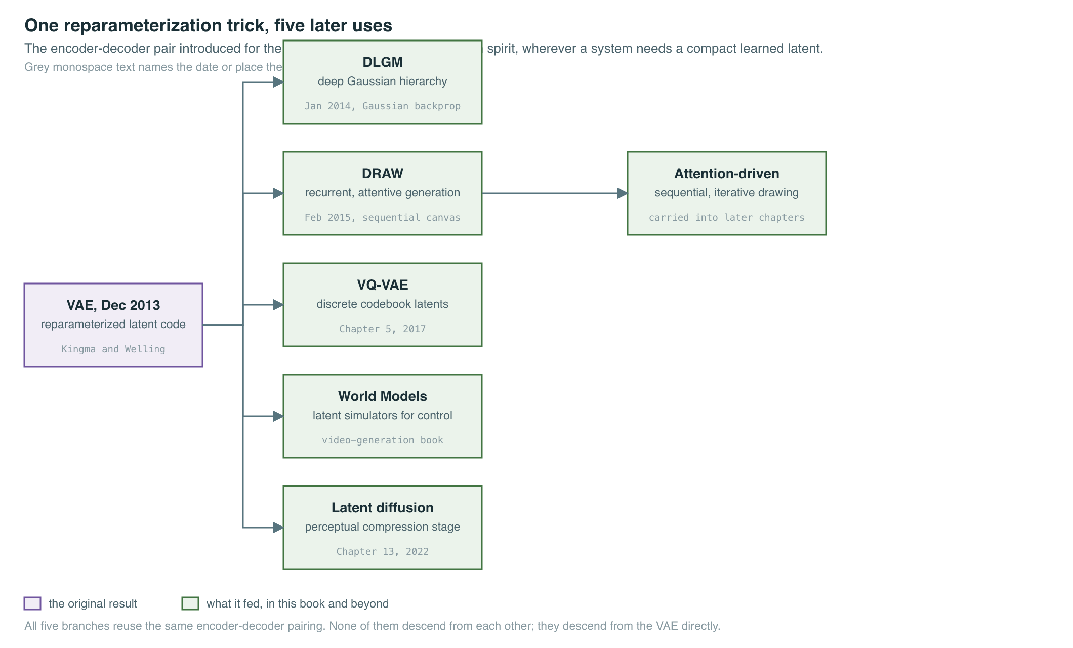
The lineage from here runs in several directions this book returns to. The discrete-latent counterpart to this chapter’s continuous Gaussian codes — VQ-VAE’s learned codebook — is covered in Pixels One at a Time. The evidence lower bound itself, generalized from a single denoising step to a full noise-adding Markov chain, becomes the training objective for diffusion models in Diffusion Foundations — a different generative mechanism built on the same inequality proved above. The perceptual-compression autoencoder sitting in front of every Stable Diffusion forward pass, turning a 512-pixel image into a small latent grid before diffusion ever runs, descends architecturally from the encoder-decoder pairing introduced here, as described in Latent Diffusion and Stable Diffusion. Outside this book, the same VAE block became the perception component of learned world models for control and simulation, a thread picked up in Predicting the Next Frame. And the alternative path taken by adversarial training, published within the same year, is the subject of The Adversarial Game.

Key Papers

Paper	Authors	Year	Link	Why it matters
Auto-Encoding Variational Bayes	Kingma & Welling	2013	arXiv:1312.6114	Introduces the reparameterization trick, the SGVB estimator, and the term “variational auto-encoder”
Stochastic Backpropagation and Approximate Inference in Deep Generative Models	Rezende, Mohamed & Wierstra	2014	arXiv:1401.4082	Independently derives the same reparameterization from Gaussian gradient identities; generalizes to deep latent Gaussian models
DRAW: A Recurrent Neural Network For Image Generation	Gregor, Danihelka, Graves, Rezende & Wierstra	2015	arXiv:1502.04623	Extends the VAE to a recurrent, differentiably-attentive process; best 2015 result on binarized MNIST