Diffusion Foundations

It is June 2020. Generative adversarial networks have spent six years winning every image-quality contest through an adversarial minimax game that produces sharp samples but resists stable training, while variational autoencoders offer tractable, likelihood-based optimization at the cost of blurry output. A three-author paper out of UC Berkeley revives an idea first sketched five years earlier and largely ignored since: destroy an image with noise in small increments, then train a single network to undo that damage one increment at a time. The resulting model matches state-of-the-art GAN image quality on CIFAR-10 with no discriminator, no adversarial loss, and none of the training instability that comes with them.

Where We Were

By the middle of the 2010s, generative image modeling had split into two families, and each owned one half of what a good model needed. The variational autoencoder (Variational Autoencoders), introduced in December 2013, trained an encoder-decoder pair by maximizing a tractable lower bound on data likelihood — the evidence lower bound, or ELBO — giving stable, well-understood optimization with an explicit probabilistic objective. Its cost was visual: the Gaussian assumptions and the averaging effect of maximum-likelihood training under that bound produced samples that were recognizable but soft, missing the high-frequency detail a photograph has.

The generative adversarial network (Generative Adversarial Networks), introduced six months later in June 2014, took the opposite trade. A generator and a discriminator played a minimax game with no explicit likelihood at all, and the resulting samples were sharp. But the adversarial objective was notoriously unstable to optimize, prone to mode collapse — the generator learning to produce a narrow slice of the data distribution rather than its full diversity — and sensitive enough to hyperparameters that stabilizing it became its own multi-year research program: WGAN’s Wasserstein objective in January 2017, WGAN-GP’s gradient penalty two months later, and a run of architectural fixes through ProGAN’s progressive growing in October 2017 (Taming GAN Training). By BigGAN in September 2018 and StyleGAN in December 2018, adversarially trained models were producing high-fidelity images at scale — but the field had spent four years learning to tame one specific training pathology rather than eliminating it (The GAN Golden Age).

Buried in this period was a third approach that neither camp noticed. In March 2015, a paper inspired by non-equilibrium statistical physics proposed a different way to build a tractable generative model: define a forward process that “systematically and slowly” destroys the structure of a data distribution through repeated small steps of noise, and train a neural network to learn the reverse process that restores it, step by step (Sohl-Dickstein et al., 2015). The paper demonstrated the idea on toy two-dimensional data, MNIST digits, and small natural-image datasets, showing it was possible to learn, sample from, and evaluate probabilities under a model built this way — but it produced nothing resembling GAN-quality images, and against the ProGAN and BigGAN results filling ICLR and NeurIPS proceedings later in the decade, it read as a mathematical curiosity rather than a competitor. For four years it stayed that way, cited occasionally, applied by almost no one.

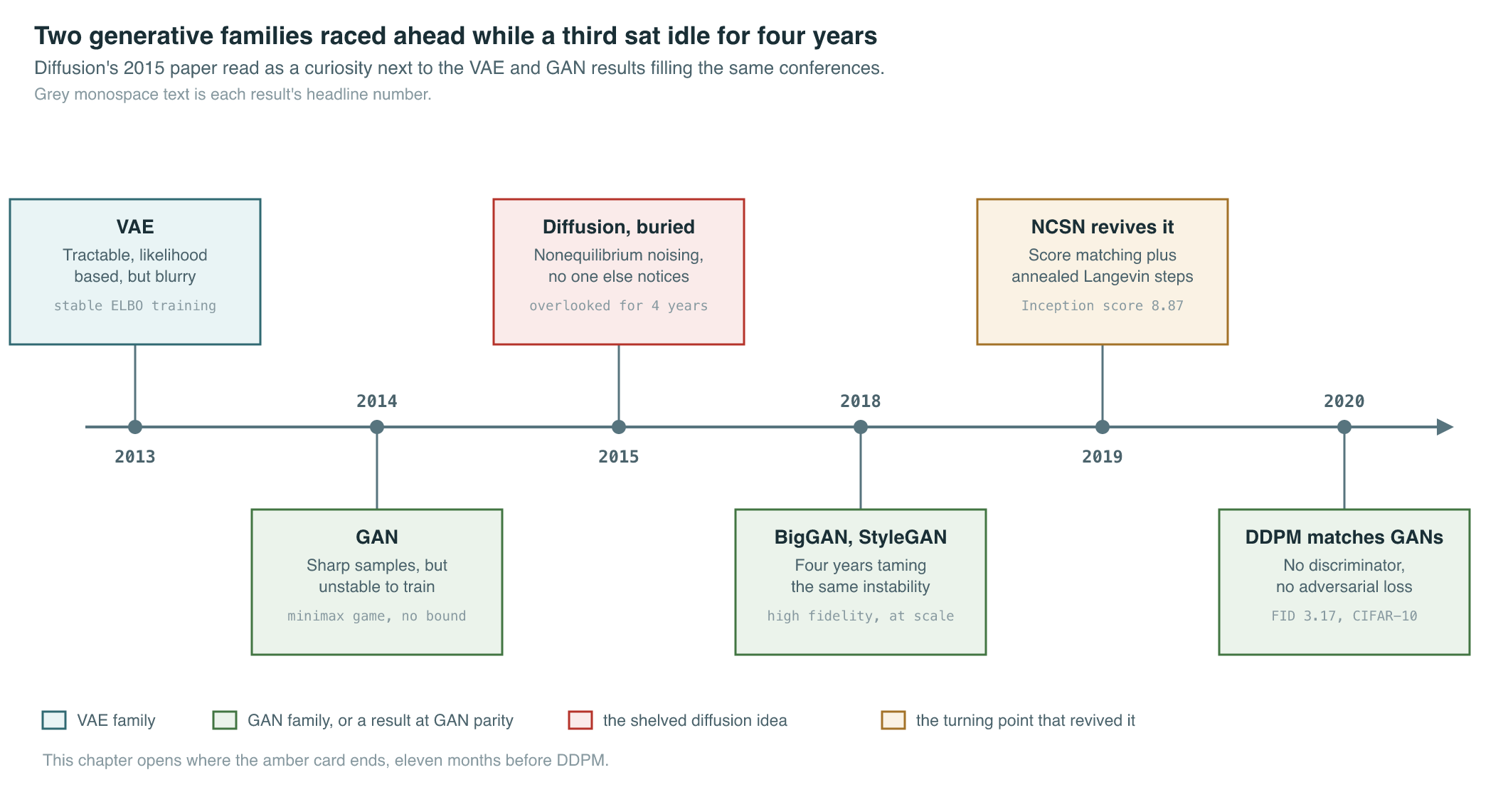
The question sitting unanswered at the end of the 2010s was whether a third path existed: a model with the stable, likelihood-based training of a VAE, but the sample quality of a GAN. Two papers, four years apart in origin but only eleven months apart in publication, would answer it.

The Breakthrough

The revival began from a different mathematical direction than Sohl-Dickstein et al. had taken. In July 2019, Song and Ermon proposed generating samples not by learning a full generative model at all, but by learning the score function — the gradient of the log data density, $\nabla_x \log p(x)$ — and then using that gradient to walk samples toward high-density regions via Langevin dynamics, a sampling procedure borrowed from statistical physics (Song & Ermon, 2019). Their Noise Conditional Score Network, or NCSN, solved a problem that had stalled earlier score-based attempts: raw data lives on a low-dimensional manifold inside a much higher-dimensional pixel space, where the true score function is undefined off-manifold and poorly estimated on it. NCSN’s fix was to perturb the data with Gaussian noise at several different scales and train one network to estimate the score at every scale jointly, then sample by annealing — running Langevin dynamics starting from a large noise scale and gradually decreasing it as the sample approaches the data manifold. The paper reported that its models “produce samples comparable to GANs on MNIST, CelebA and CIFAR-10,” reaching an Inception Score of 8.87 on CIFAR-10, using a method the paper describes as requiring “no sampling during training or the use of adversarial methods” — no discriminator to train or destabilize.

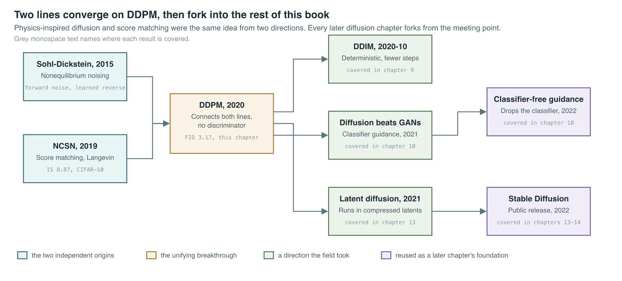
NCSN and the 2015 diffusion paper had converged on the same shape of solution — corrupt data with noise, then learn to undo the corruption — from opposite theoretical starting points: one from probabilistic latent-variable modeling, the other from score matching and physics-inspired sampling. Eleven months after NCSN, Ho, Jain, and Abbeel connected the two lines explicitly. Their Denoising Diffusion Probabilistic Model, or DDPM, is a direct descendant of Sohl-Dickstein et al.’s forward-and-reverse Markov chain, but it is trained using “a novel connection between diffusion probabilistic models and denoising score matching with Langevin dynamics” — the same score-based idea NCSN had put to work independently (Ho et al., 2020).

The mechanism, described narratively before the equations arrive in the next section: take a real image and add a small, fixed amount of Gaussian noise to it, repeat that a thousand times, and the image becomes indistinguishable from pure noise. That forward process needs no learning at all — it is a fixed schedule. The learning happens in reverse: train a single neural network to look at a noisy image at step $t$ and predict what noise was added, so that subtracting the prediction recovers a slightly less noisy image at step $t-1$. Run the trained network a thousand times, starting from pure noise, and it walks backward all the way to a plausible image the network has never seen before. Ho et al. used a U-Net styled after an unmasked PixelCNN++, with group normalization throughout, self-attention at the $16 \times 16$ feature-map resolution, and a Transformer-style sinusoidal embedding to tell the shared network which timestep $t$ it is currently denoising.

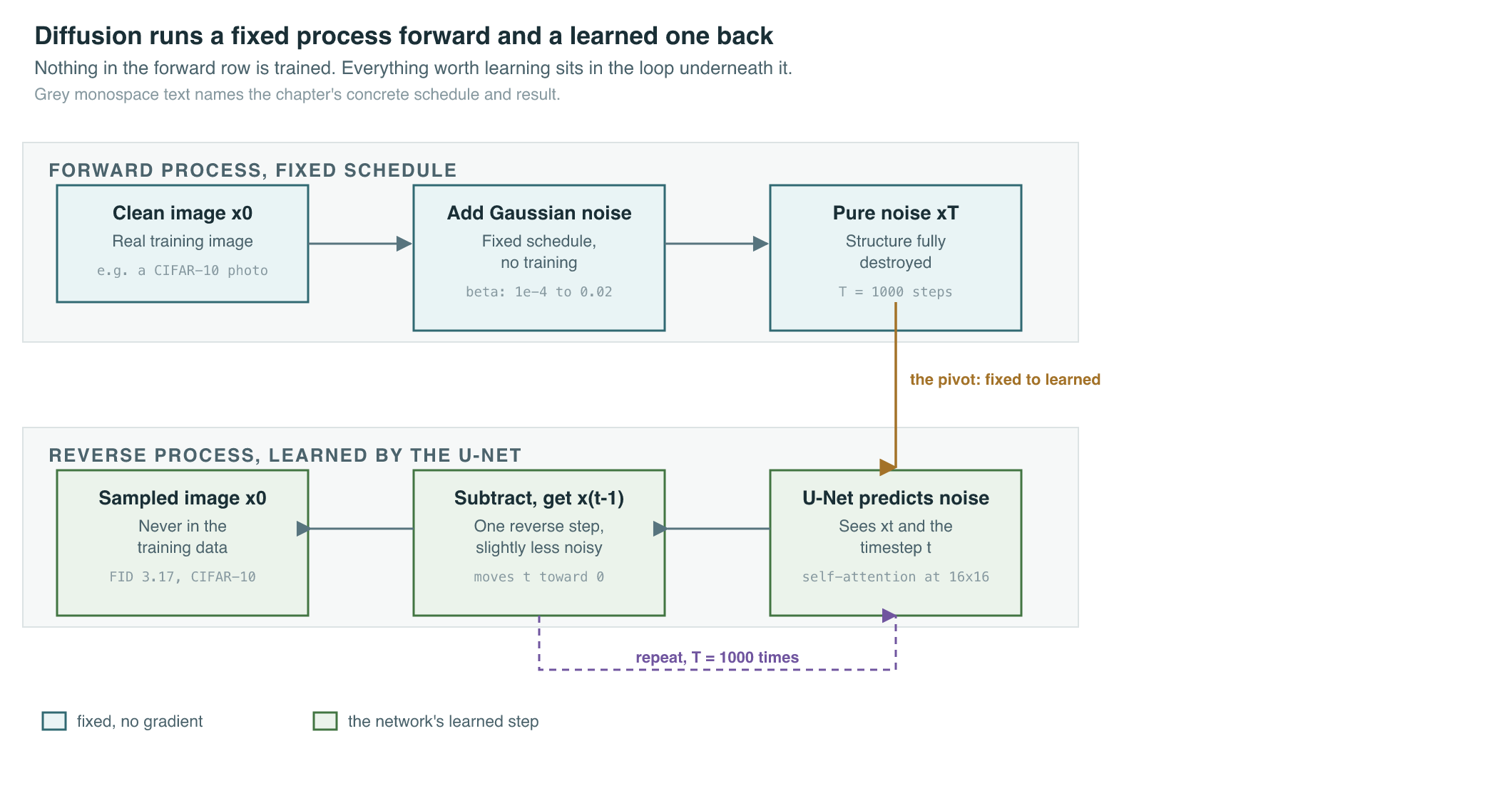
The result was decisive on the axis that mattered: unconditional CIFAR-10 generation reached a Fréchet Inception Distance of 3.17 and an Inception Score of 9.46, which the paper describes as state of the art for the metric at the time, produced by a model with no discriminator, no adversarial loss, and no mode-collapse failure mode to manage. The paper also showed that its training objective, once simplified, could be interpreted as “a generalization of autoregressive decoding” — a progressive decompression of an image out of noise, one step at a time.

The Mathematics

Notation follows Ho, Jain & Abbeel (2020). The forward process turns a data sample $x_0$ into a sequence of increasingly noisy versions $x_1, \dots, x_T$ through a fixed Markov chain with no learned parameters:

$$q(x_t \mid x_{t-1}) = \mathcal{N}\!\left(x_t;\ \sqrt{1-\beta_t}\, x_{t-1},\ \beta_t \mathbf{I}\right)$$

Because each step is Gaussian, the whole chain has a closed form: any noisy version $x_t$ can be sampled directly from the original image $x_0$ without simulating every intermediate step.

$$\begin{aligned} q(x_t \mid x_0) &= \mathcal{N}\!\left(x_t;\ \sqrt{\bar\alpha_t}\, x_0,\ (1-\bar\alpha_t)\mathbf{I}\right) \\ x_t &= \sqrt{\bar\alpha_t}\, x_0 + \sqrt{1-\bar\alpha_t}\, \epsilon, \qquad \epsilon \sim \mathcal{N}(0,\mathbf{I}) \end{aligned}$$

Symbol	Meaning
$x_0$	the original, clean data sample
$x_t$	the sample after $t$ steps of forward noising
$\beta_t$	fixed noise-variance schedule at step $t$, $10^{-4}$ to $0.02$ across $T=1000$ steps
$\bar\alpha_t$	cumulative product $\prod_{s=1}^{t}(1-\beta_s)$, the fraction of original signal remaining
$\epsilon$	standard Gaussian noise, the quantity the network learns to predict

Generation runs the chain backward. The true reverse step $q(x_{t-1}\mid x_t)$ is intractable to compute directly because it would require knowing $x_0$, so a neural network learns an approximation:

$$p_\theta(x_{t-1} \mid x_t) = \mathcal{N}\!\left(x_{t-1};\ \mu_\theta(x_t, t),\ \Sigma_\theta(x_t, t)\right)$$

Symbol	Meaning
$p_\theta$	the learned reverse-process distribution, parameterized by network weights $\theta$
$\mu_\theta(x_t, t)$	network-predicted mean of the previous, less-noisy step
$\Sigma_\theta(x_t, t)$	network-predicted (or fixed) variance of that step
$\theta$	the trainable parameters of the U-Net

Training minimizes a variational bound on the negative log-likelihood — the diffusion-specific instance of the evidence lower bound taught in full in the VAE chapter:

$$\mathbb{E}_q\!\left[-\log p_\theta(x_0)\right] \;\le\; \mathbb{E}_q\!\left[-\log p(x_T) - \sum_{t \ge 1} \log \frac{p_\theta(x_{t-1}\mid x_t)}{q(x_t \mid x_{t-1})}\right] \;=:\; L$$

Symbol	Meaning
$L$	the variational bound being minimized — the training objective
$p(x_T)$	the fixed prior at the end of the forward chain, standard Gaussian noise
$q(\cdot)$	the fixed forward process, defining the “target” the reverse process is trained to match

Ho, Jain, and Abbeel’s central contribution was showing that $L$, after re-deriving $\mu_\theta$ in terms of a noise-prediction network $\epsilon_\theta$ and re-weighting its terms, collapses to a strikingly plain regression loss — the equation concept-ownership in this book calls simply the DDPM loss:

$$L_{\mathrm{simple}}(\theta) := \mathbb{E}_{t,\, x_0,\, \epsilon}\left[\left\lVert \epsilon - \epsilon_\theta\!\left(\sqrt{\bar\alpha_t}\, x_0 + \sqrt{1-\bar\alpha_t}\, \epsilon,\ t\right) \right\rVert^2\right]$$

Symbol	Meaning
$L_{\mathrm{simple}}$	the simplified training loss — an unweighted mean-squared-error regression
$\epsilon_\theta(\cdot,\ t)$	the U-Net’s predicted noise, given a noisy input and timestep $t$
$t$	a timestep sampled uniformly from $1, \dots, T$ at each training step
$x_0,\ \epsilon$	a training image and the random Gaussian noise mixed into it

The score-based line from NCSN and the probabilistic line from Sohl-Dickstein and DDPM turn out to be the same objective in disguise. A noise-prediction network trained on $L_{\mathrm{simple}}$ is, up to a known scaling factor, also an estimate of the score function NCSN trains directly:

$$s_\theta(x_t, t) := \nabla_{x_t} \log p(x_t) \;\approx\; -\,\frac{\epsilon_\theta(x_t, t)}{\sqrt{1-\bar\alpha_t}}$$

Symbol	Meaning
$s_\theta(x_t, t)$	the network’s implied estimate of the score at noise level $t$
$\nabla_{x_t} \log p(x_t)$	the true score — gradient of log-density with respect to the noisy sample
$\epsilon_\theta(x_t, t)$	the same noise-prediction network trained on $L_{\mathrm{simple}}$
$\sqrt{1-\bar\alpha_t}$	the rescaling factor connecting the two parameterizations

What It Enabled

The immediate consequence was a second viable path to GAN-competitive image quality, this time built on a training procedure with no adversarial component to destabilize. The following table lines up the trade-offs the field had been managing for six years against the one diffusion introduced.

	VAE	GAN	Diffusion, 2020
Training signal	one closed-form bound, the ELBO	two competing networks, minimax game	one closed-form regression loss, $L_{\mathrm{simple}}$
Training stability	stable	prone to mode collapse and divergence	stable, no adversarial dynamics
Sample quality (2020)	blurry	best available (BigGAN, StyleGAN2)	matches best GANs on CIFAR-10, FID 3.17
Likelihood / density estimate	explicit lower bound	none	explicit variational bound
Cost to generate one sample	one decoder forward pass	one generator forward pass	up to $T=1000$ sequential network passes

That last row was diffusion’s most consequential weakness, and the field went after it almost immediately: reducing the number of sampling steps without discarding the trained model became the subject of the very next chapter’s deterministic samplers (Scores, SDEs, and Faster Sampling) and, later, of dedicated few-step and single-step distillation techniques (Few-Step Generation).

Sample-quality gains followed on a short timeline once the recipe existed. Within a year, diffusion models were shown to outperform GANs on ImageNet-scale image fidelity, a result covered in this book’s chapter on classifier guidance (Guidance), reversing six years of GAN dominance on the field’s headline benchmark. Within eighteen months, running the diffusion process in a pretrained autoencoder’s compressed latent space rather than raw pixels made the same recipe cheap enough to train and run at consumer scale, the foundation under Stable Diffusion (Latent Diffusion and Stable Diffusion).

Key Papers

Paper	Authors	Year	Link	Why it matters
Deep Unsupervised Learning using Nonequilibrium Thermodynamics	Sohl-Dickstein, Weiss, Maheswaranathan, Ganguli	2015	arXiv:1503.03585	First forward-noise, learned-reverse-process generative model; overlooked for four years but the structural ancestor of every later diffusion model
Generative Modeling by Estimating Gradients of the Data Distribution	Song, Ermon	2019	arXiv:1907.05600	Revived denoising-based generation via score matching and annealed Langevin dynamics; reached Inception Score 8.87 on CIFAR-10 with no adversarial training
Denoising Diffusion Probabilistic Models	Ho, Jain, Abbeel	2020	arXiv:2006.11239	Reduced the training objective to a simple noise-prediction regression and connected it to score matching; FID 3.17 on CIFAR-10 made diffusion GAN-competitive

PM Lens