The Adversarial Game

It is June 2014. Generative models can approximate a data distribution and sample from it, but every existing recipe pays for that ability with an intractable sum, a Markov chain, or an approximate posterior. A paper out of the Université de Montréal proposes training two networks against each other instead of training one network to fit a likelihood — a generator producing samples, a discriminator judging them — and the resulting adversarial game becomes, for the next seven years, the dominant way to make a neural network produce a convincing image.

Where We Were

By 2014 the field had two established families for learning a distribution over images, and both carried a structural tax. Undirected graphical models — restricted Boltzmann machines and the deep belief nets built by stacking them (engine room, Chapter 1 covers their layer-wise pretraining) — represent probability as the product of unnormalized potential functions divided by a partition function, a global sum over every possible configuration of the model’s variables. That partition function, and its gradient, is intractable for anything but the smallest models; fitting one in practice means running Markov chain Monte Carlo and hoping the chain mixes well enough to be useful, a hope that gets harder to sustain as the model grows.

Directed latent-variable models sidestepped the partition function but ran into a different wall: the posterior over latent variables, needed to fit the model by maximum likelihood, is itself intractable for anything but the simplest priors and likelihoods. The variational autoencoder, published six months earlier, addressed this by learning an approximate posterior and optimizing a tractable lower bound on the likelihood instead of the likelihood itself — the ELBO, whose derivation is owned by Chapter 2. The VAE worked, and it needed no Markov chain, but the bound it optimized was a bound, not the true likelihood, and in practice its samples came out characteristically blurry — the cost of an explicit, tractable density.

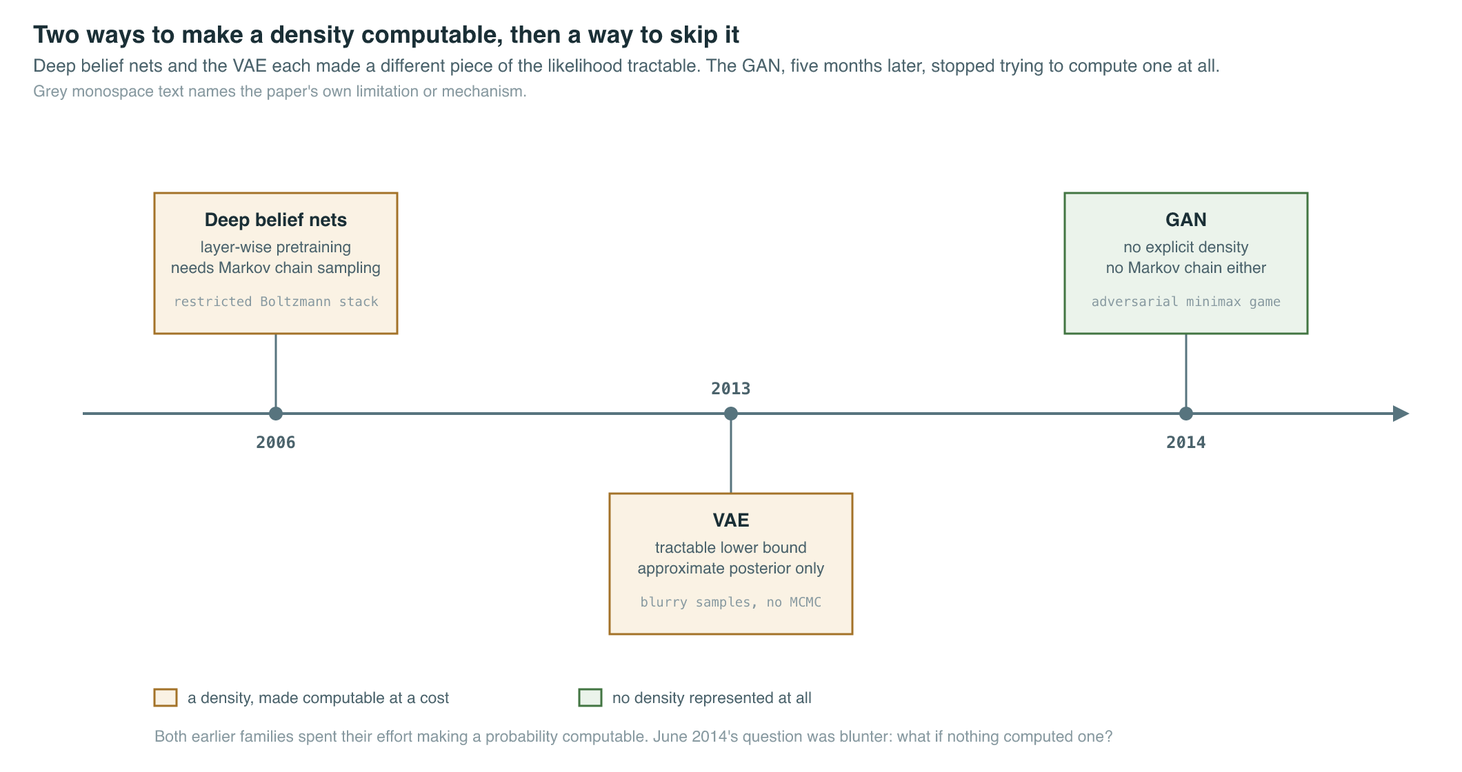
Both families, in other words, spent their effort making an explicit probability computable — by approximating a partition function, or by bounding a likelihood — and both paid for that explicitness with either sampling difficulty or approximation error. The question the next paper asked was blunter: what if the model never represented a probability density at all, and was judged only on whether the samples it produced were any good?

The Breakthrough

Generative Adversarial Networks (Goodfellow et al., 2014) frames generative modeling as a two-player game rather than a density-fitting problem. A generator network $G$ maps noise $z$, drawn from a simple fixed prior, to a point in data space, trying to produce samples indistinguishable from real data. A discriminator network $D$ looks at a sample — real or generated — and outputs the probability that it came from the real data rather than from $G$. The two are trained simultaneously: $D$ is pushed to get better at telling real from fake, and $G$ is pushed to get better at fooling $D$. The paper’s own analogy is counterfeiting: the generator is a team of forgers, the discriminator is the police trying to spot the forgeries, and competition between the two drives the forgeries toward indistinguishable from genuine currency.

Neither network needs to represent a probability density anywhere. $G$ is a differentiable function — in the original paper, a multilayer perceptron — with no tractable expression for the density of the samples it produces; it is defined entirely by the transformation it applies to noise. $D$ is a second multilayer perceptron trained as an ordinary binary classifier. Both are trained purely by backpropagation, with no Markov chain during training and no approximate inference network needed to invert the generator. Sampling, at the end, is one forward pass through $G$.

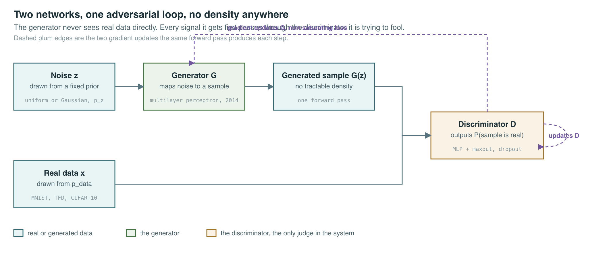
Training alternates rather than solving the game exactly at each step: optimizing $D$ to convergence inside every generator update would be computationally prohibitive and, on a finite dataset, would overfit. The paper’s Algorithm 1 instead runs $k$ gradient-ascent steps on $D$ for every one gradient-descent step on $G$ — the authors used $k=1$, the cheapest option — updating both with ordinary minibatch stochastic gradient descent with momentum. A second practical adjustment mattered as much as the algorithm itself: early in training, when $G$ is still poor, $D$ rejects generated samples with high confidence, and the generator’s intended loss saturates and stops providing a useful gradient. Rather than have $G$ minimize that saturating term, the authors trained it to maximize a differently-shaped objective with the same fixed point but a much stronger gradient early on — the “non-saturating” heuristic loss used by nearly every GAN trained since.

The 2014 experiments used multilayer perceptrons for the generator — a mix of rectifier and sigmoid units — and a discriminator built from maxout units with dropout applied during training, across three datasets: MNIST, the Toronto Face Database, and CIFAR-10. Because the model has no tractable likelihood, the authors evaluated it by fitting a Gaussian Parzen window to generated samples and reporting the log-likelihood of the test set under that window — a noisy but standard proxy at the time. The adversarial net scored a mean log-likelihood of 225 ± 2 on MNIST and 2057 ± 26 on the Toronto Face Database, ahead of a deep belief net (138 ± 2 / 1909 ± 66) and a deep generative stochastic network (214 ± 1.1 / 1890 ± 29), and within range of a stacked contractive autoencoder (121 ± 1.6 / 2110 ± 50, the best TFD score in the comparison). The code — implemented in Theano, the Python library that could already compile the same numerical graph to either a CPU or a GPU backend — was released publicly alongside the paper.

The paper’s own discussion of the framework’s disadvantages named the failure mode that would define the next several years of GAN research, without yet solving it. Because $G$ is only ever updated through gradients flowing back from $D$, and never sees real data directly, nothing forces it to cover the full diversity of $p_{\mathrm{data}}$. The authors called the extreme case the “Helvetica scenario”: $G$ collapses many different values of $z$ onto the same output $x$, sacrificing diversity for a sample that reliably fools the current discriminator — much as the negative-phase chains in a Boltzmann machine can go stale if not refreshed often enough during learning. This is mode collapse, and the paper flags it as an open synchronization problem between $G$ and $D$ rather than a solved one; Chapter 4 covers the training-stabilization work — DCGAN, WGAN, WGAN-GP — that spent the following three years attacking it directly.

Five months later, a short follow-up showed how easily the framework generalized. Conditional Generative Adversarial Nets (Mirza and Osindero, 2014) extended the game by feeding auxiliary information $y$ — a class label, in the simplest case — into both networks: the generator now maps $z$ conditioned on $y$, and the discriminator judges $x$ conditioned on $y$. On MNIST, conditioning on the one-hot class label let the generator produce digits of a chosen class on demand, at the cost of a lower Parzen-window score (132 ± 1.8) than the unconditional model, which the authors reported candidly as a proof of concept rather than a state-of-the-art result. A second experiment conditioned generation on image features from a pretrained convolutional network to generate word-vector tags for photographs from the MIR Flickr 25,000 dataset — an early demonstration that the same mechanism could bridge two different modalities, years before that idea became central to text-to-image generation (covered from Chapter 7 onward).

The Mathematics

The generator and discriminator play a two-player minimax game over a single value function:

$$\min_G \max_D V(D, G) = \mathbb{E}_{x \sim p_{\mathrm{data}}(x)}\big[\log D(x)\big] + \mathbb{E}_{z \sim p_z(z)}\big[\log\big(1 - D(G(z))\big)\big]$$

Symbol	Meaning
$D(x)$	discriminator’s output — estimated probability that $x$ is real
$G(z)$	generator’s output — a sample produced from noise $z$
$p_{\mathrm{data}}(x)$	the true data distribution
$p_z(z)$	the fixed noise prior, e.g. uniform or Gaussian
$\mathbb{E}$	expectation, i.e. an average over the given distribution

Holding $G$ fixed, the value function has a closed-form optimal discriminator:

$$D^{*}_{G}(x) = \frac{p_{\mathrm{data}}(x)}{p_{\mathrm{data}}(x) + p_g(x)}$$

Substituting $D^{*}_G$ back into $V$ and simplifying gives a criterion, $C(G) = \max_D V(D,G)$, whose global minimum the paper proves occurs exactly when $p_g = p_{\mathrm{data}}$, with value $-\log 4$. Rewriting that criterion in terms of the Kullback–Leibler divergence and recognizing the Jensen–Shannon divergence inside it gives the result the field still cites:

$$C(G) = -\log 4 + 2 \cdot \mathrm{JSD}\big(p_{\mathrm{data}} \,\|\, p_g\big)$$

Symbol	Meaning
$C(G)$	the value of the game once $D$ has been optimized for the current $G$
$\mathrm{JSD}(\cdot \,\|\, \cdot)$	Jensen–Shannon divergence between two distributions
$p_{\mathrm{data}}$	the true data distribution
$p_g$	the distribution induced by the current generator

In practice, the training signal for $G$ swaps to the non-saturating form as soon as $D$ is confident, replacing $\min_G \log(1-D(G(z)))$ with $\max_G \log D(G(z))$ — the same fixed point, a steeper gradient when $G$ is weak. The conditional variant folds an auxiliary variable $y$ into every term of the same game:

$$\min_G \max_D V(D, G) = \mathbb{E}_{x \sim p_{\mathrm{data}}(x)}\big[\log D(x \mid y)\big] + \mathbb{E}_{z \sim p_z(z)}\big[\log\big(1 - D(G(z \mid y))\big)\big]$$

Symbol	Meaning
$y$	the conditioning variable — a class label or other auxiliary information
$D(x \mid y)$	discriminator’s probability that $x$ is real, given $y$
$G(z \mid y)$	generator’s output given noise $z$ and condition $y$
$p_{\mathrm{data}}(x)$, $p_z(z)$	the data distribution and noise prior, as above
$\mathbb{E}$	expectation over the given distribution

What It Enabled

The GAN paper itself was explicit about where its framework sat relative to the alternatives, and its own comparison — reproduced here in condensed form — is worth keeping because it names the trade-off precisely:

Operation	Deep directed graphical models	Deep undirected graphical models	Adversarial nets
Inference during training	Needed, approximate	Needed, MCMC-based	Not needed
Sampling	No difficulties	Requires a Markov chain	No difficulties
Evaluating $p(x)$	Intractable, approximated	Intractable, approximated	Not explicitly represented
Model design constraint	Nearly all models incur difficulty	Careful design needed	Any differentiable function permitted

Set against the VAE specifically, the trade is sharper still: the VAE keeps an explicit, tractable (bounded) density and pays for it with blur; the GAN drops the density entirely and, freed from ever having to reconstruct or bound a likelihood, produced qualitatively sharper samples from the start — at the cost of an unstable training procedure and no way to measure how well it was actually covering the true distribution.

	VAE (Chapter 2)	GAN (this chapter)
Density	Explicit, via a tractable lower bound (ELBO)	Implicit — never computed
Training signal	Reconstruction plus KL regularizer, single network	Adversarial minimax game, two networks
Sample sharpness (2013–2014)	Characteristically blurry	Comparatively sharp, but unstable to train
Known failure mode	Overly smooth, low-detail samples	Mode collapse, non-convergence
Likelihood evaluation	Direct (bound)	Only approximate, e.g. Parzen windows

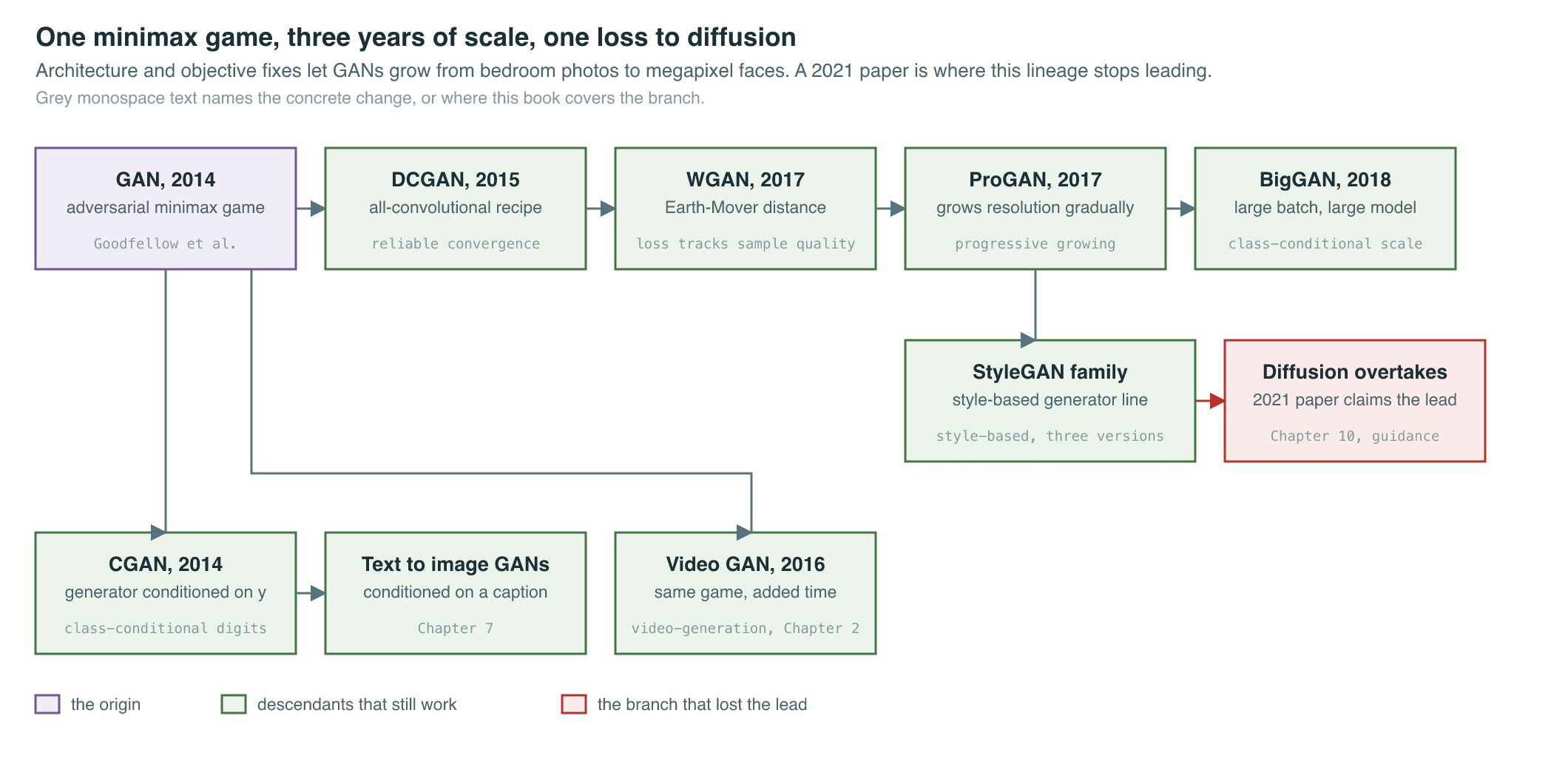
The theoretical result — that the adversarial game minimizes the Jensen–Shannon divergence at its equilibrium — turned out to describe an equilibrium that ordinary gradient descent on two competing networks rarely reaches exactly, and the following three years of GAN research were substantially about closing that gap between theory and practice. Convolutional architectures replaced the original multilayer perceptrons with DCGAN in November 2015; alternative divergences replaced Jensen–Shannon with the Wasserstein distance in January 2017, followed by a gradient-penalty variant in March 2017 to fix a remaining instability — all covered in Chapter 4. Once training was tamed, scale and fidelity became the frontier: progressive growing in October 2017, then BigGAN in September 2018, then the style-based generator line — StyleGAN, StyleGAN2, and StyleGAN3 — running from December 2018 through June 2021, all in Chapter 6. The conditional mechanism from this chapter became the entry point for text-conditioned generation, first with stacked and attention-based text-to-image GANs in Chapter 7, and the same adversarial idea was carried into the temporal domain by video GANs from 2016 onward, taught in Video Generation, Chapter 2. Judging any of this progress required a better metric than a Parzen window; the Fréchet Inception Distance, introduced in 2017, is covered in Chapter 21. The adversarial approach held the state of the art in raw image fidelity through the rest of the 2010s, until a 2021 paper made the explicit claim that diffusion models — the subject of Chapter 8 — had overtaken it, a turning point covered in Chapter 10.

Key Papers

Paper	Authors	Year	Link	Why it matters
Generative Adversarial Networks	Goodfellow et al.	2014	arXiv:1406.2661	Introduces the adversarial minimax game — a generator and discriminator trained against each other with no explicit density and no Markov chain — and proves its equilibrium minimizes the Jensen–Shannon divergence
Conditional Generative Adversarial Nets	Mirza and Osindero	2014	arXiv:1411.1784	Extends the adversarial game with an auxiliary conditioning variable fed to both networks, the mechanism every later text-to-image and class-conditional GAN builds on

PM Lens