The Generative Problem

It is 2006. A neural network with a bottleneck eleven times narrower than its input learns to compress a handwritten digit down to thirty numbers and reconstruct it more faithfully than three decades of linear methods had managed. Nothing about that network, however, defines a probability distribution it can draw a fresh digit from — it can only echo back what it is shown. The gap between compressing what already exists and generating what could exist is the subject of this chapter, and of most of the book that follows.

Where We Were

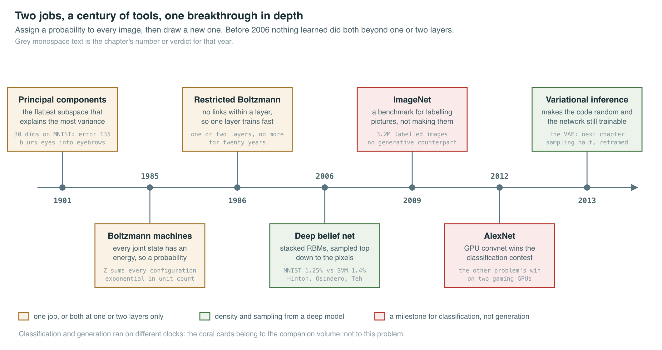
A generative model of images has two jobs, and before 2006 no method did both of them well on anything resembling a photograph. The first job is density estimation: assign a number, $p(x)$ , to every possible image $x$ , high for images that look like the training data and low for images that do not. The second job is sampling: actually produce a new $x$ drawn from that distribution, one that was not in the training set but is recognizably the same kind of thing. A histogram over pixel values can estimate a crude density. A lookup table can “sample” by replaying training examples. Neither does anything a person would call imagining a picture.

The classical toolkit for the first job was built on Gaussian assumptions. Principal component analysis (PCA) finds the linear subspace that captures the most variance in a dataset and treats deviation from that subspace as noise; a mixture of Gaussians extends the same idea to a handful of clusters. Both are density estimators in a strict sense — each assigns a likelihood to a data point — and both are exactly solvable with linear algebra, no iterative training required. Natural images defeat them for a simple structural reason: the manifold of “images that look like faces” or “images that look like handwritten sevens” is nonlinear, curved through pixel space in a way no flat subspace or bell-curve cluster can trace. Compressing a face to thirty numbers with PCA blurs the eyes into the eyebrows; the linear model has no way to represent that a rotated nose and a shifted mouth are both small, structured changes rather than large, unstructured ones.

The alternative toolkit, older than PCA in one sense and newer in its practical form, was the Boltzmann machine: a network of binary units connected by symmetric weights, in which every joint configuration of units has an energy, and every configuration’s probability is a simple function of that energy. Unlike PCA, a Boltzmann machine can in principle do both jobs — it defines a genuine joint distribution over its units, and that distribution can be sampled by letting the network settle stochastically toward low-energy states. In practice, training a general Boltzmann machine required a form of statistical estimation that scaled miserably with the number of units, and stacking several layers of them to build a deep model made the required sampling exponentially harder still. Restricting the connections so that no two visible units and no two hidden units connect to each other — the restricted Boltzmann machine (RBM) — made a single layer tractable to train with a fast approximate procedure. Composing several such layers into something deep remained, through the 1980s and 1990s, a problem without a practical answer. Layer count in generative models of images stayed at one or two.

Two further pieces of context, dated precisely by the master timeline: the ImageNet dataset would not be published until 2009, and the GPU-trained convolutional network that would win a competition built on it would not arrive until 2012. Both belong to a different problem — classifying images into categories — that this book’s companion volume covers from the hardware side. The generative problem this chapter tracks ran on a slower clock, waiting less for a bigger dataset than for a way to train something deeper than one or two layers of Boltzmann units.

A century of density estimators and one breakthrough in depth. The coral cards belong to the classification problem and the companion volume; the generative problem ran on its own, slower clock. PNG ↓

The Breakthrough

In 2006, three researchers at the University of Toronto solved the depth problem for Boltzmann-style generative models, and a fourth collaboration from the same lab reused the solution for a narrower, non-generative purpose — and the contrast between the two turned out to be more instructive than either result alone.

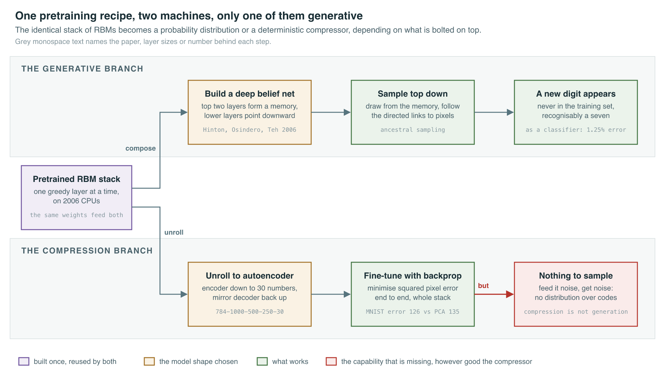
Geoffrey Hinton, Simon Osindero, and Yee-Whye Teh showed that a stack of RBMs, each trained on the hidden-unit activities produced by the layer below it, can be composed into a single deep model — a deep belief net (DBN) — whose top two layers form an undirected associative memory and whose lower layers form a chain of directed generative connections down to the pixels (Hinton, Osindero, and Teh, 2006). The greedy, layer-by-layer training procedure sidesteps the intractable joint estimation that had stalled deep Boltzmann machines for two decades, and the paper proves that adding each new layer, trained this way, is guaranteed under mild conditions to improve a bound on how well the composite model explains the training data. Fine-tuned with a contrastive version of the wake-sleep algorithm, their network classified MNIST digits with a reported 1.25 percent test error, edging out a contemporary support vector machine’s 1.4 percent — a result that helped reopen the field’s interest in deep architectures after roughly two decades in which “neural network” was mostly a term for a plateau rather than a frontier.

What made the DBN a genuine generative model, rather than merely a good classifier, is that the same network runs in reverse. Starting from a sample drawn from the top-layer associative memory and propagating downward through the directed connections produces a new, recognizable digit image that was never in the training set — ancestral sampling through a learned hierarchy, the second job of a generative model, done for the first time by a network with more than one or two effective layers. The full layer-wise training recipe, and the reason it needed one — the CPU hardware of 2006 could not have trained the deep joint model directly at any usable speed — is covered in The Hardware Lottery, which treats this same paper as a case study in algorithm and machine arriving out of step.

Geoffrey Hinton and Ruslan Salakhutdinov then pointed the identical pretraining trick at a different target. Instead of composing the stacked RBMs into a top-heavy associative memory, they unrolled the stack into a symmetric encoder-decoder — an 784-1000-500-250-30 network for 28-by-28 MNIST digits, encoding down to a 30-dimensional code and decoding back up to 784 pixels — and fine-tuned the whole thing end to end with ordinary backpropagation to minimize reconstruction error (Hinton and Salakhutdinov, 2006). On MNIST test images, the resulting deep autoencoder reached an average squared reconstruction error of 126 at a 30-dimensional bottleneck, against 135 for 30-dimensional PCA on the same data — a real but modest margin that mattered less than what it demonstrated: without the RBM-based layer-wise pretraining to find good starting weights, backpropagation alone gets stuck and cannot train a network this deep to reconstruct well at all. The same paper applied the technique to face images and to text-document retrieval, using the learned low-dimensional code as a compact fingerprint for nearest-neighbor lookup.

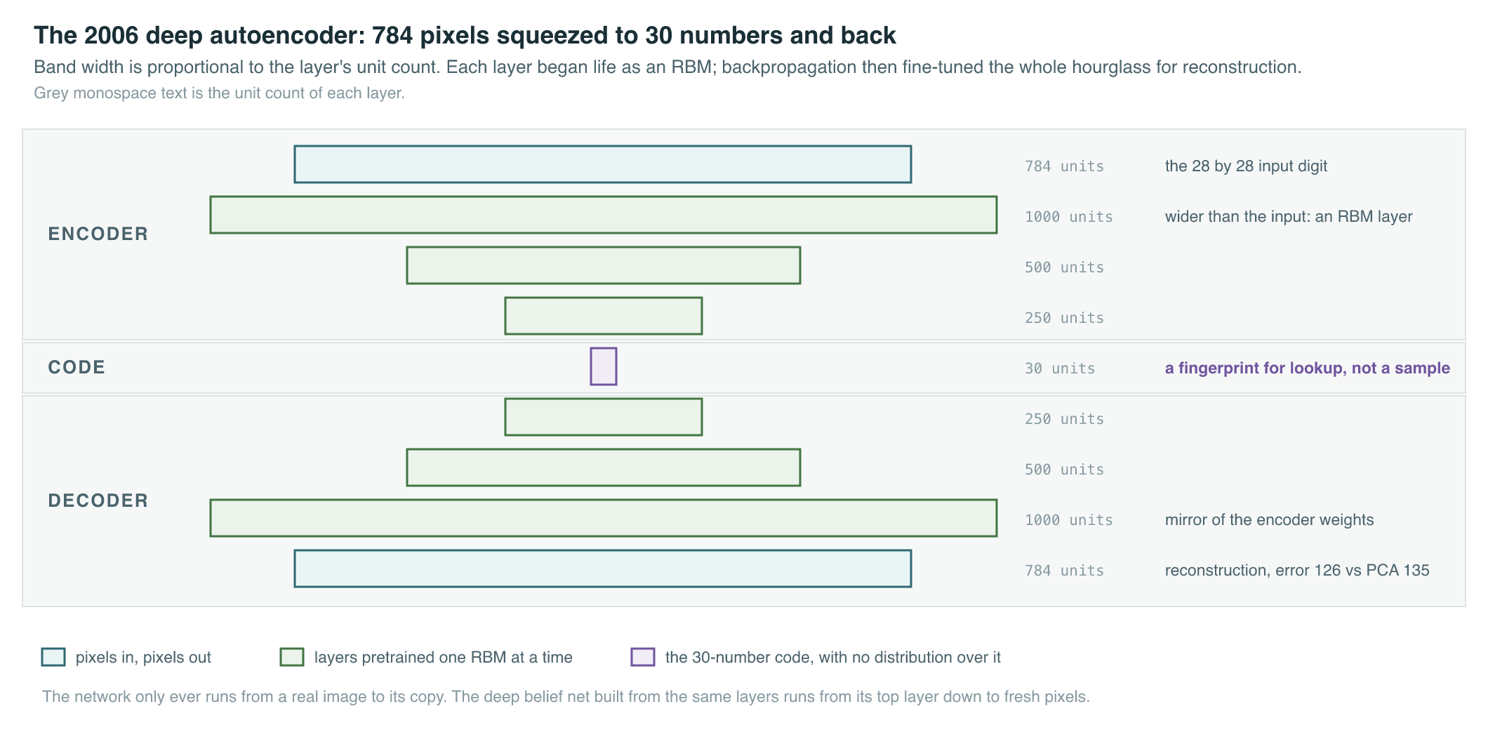
Twenty-six pixels of input for every number in the code. The hourglass is the best compressor of its day, and it only ever runs from a real image to its copy. PNG ↓

Here is the contrast the chapter is named for. The deep belief net is a probability distribution: query it for $p(x)$ , or run it forward from noise to get a new $x$ . The deep autoencoder, initialized with the exact same stack of pretrained RBMs, is a deterministic function: feed it an $x$ , get back a code and a reconstruction, and get nothing at all if you feed it noise instead of a real image — there is no probability distribution over its 30-dimensional codes to sample from. One 2006 paper solved the generative problem, in miniature, for small binary images. The other paper borrowed its machinery to build the best compressor of its day and, in doing so, made unmistakably clear that compression and generation are not the same capability, however similar the training recipes look.

The same pretrained weights, two machines. Only the branch that defines a distribution can run from noise to a new image; the better compressor cannot. PNG ↓

The Mathematics

Every generative model in this book is, at bottom, an attempt to solve the same fitting problem: choose parameters $\theta$ that make a model distribution assign high probability to observed data.

\theta^{*} = \arg\max_{\theta} \sum_{i=1}^{N} \log p_{\theta}(x_i)

Given $N$ training images $x_1, \dots, x_N$ , find the parameters $\theta$ of a model $p_\theta$ that make the training data as likely as possible under that model, measured by summing the log-probability the model assigns to each one. Maximizing a sum of logs is the same as maximizing a product of probabilities, and working in log-space keeps the arithmetic numerically stable when probabilities are very small. This buys a single, well-defined training objective — but it says nothing about whether the resulting $p_\theta$ can actually be sampled from. That second requirement, not visible in this equation, is the generative problem this chapter is named for, and every subsequent chapter’s method is a different answer to satisfying both at once.

Symbol	Meaning
$\theta$	the parameters of the model being fit
$N$	the number of training images
$x_i$	the $i$ -th training image
$p_{\theta}$	the model’s distribution over images, as a function of $\theta$

An RBM instantiates $p_\theta$ concretely, over a set of visible units $x$ (the pixels) and hidden units $h$ (learned binary features), by way of an energy function:

p(x, h) = \frac{1}{Z}\exp\left(-E(x, h)\right), \qquad E(x, h) = -a^{\top}x - b^{\top}h - x^{\top}Wh

Every joint setting of the visible units $x$ and hidden units $h$ has an energy $E(x, h)$ : low energy for configurations the model considers plausible, high energy for implausible ones. The energy itself is just three dot products — how well the biases $a$ and $b$ favor certain units being on, plus how well the weights $W$ connect visible and hidden units that tend to be on together. Exponentiating and flipping the sign turns low energy into high probability; dividing by the partition function $Z$ , the sum of $\exp(-E(x,h))$ over every possible configuration, normalizes the result into a genuine probability distribution. This single equation buys both jobs from the introduction at once — a density, $p(x) = \sum_h p(x, h)$ , and a sampling procedure, alternately resampling $x$ given $h$ and $h$ given $x$ until the pair settles into the joint distribution. The catch is $Z$ : summing over every configuration of every unit is exponential in the number of units, computable exactly only for tiny networks. That intractability is exactly why a single RBM was trained with a fast approximation rather than exact maximum likelihood, and exactly why composing several of them required the greedy, layer-by-layer recipe in The Hardware Lottery rather than joint training of the whole stack at once.

Symbol	Meaning
$x$	visible units — the observed pixels or features
$h$	hidden units — learned binary latent features
$W$	weight matrix connecting visible and hidden units
$a, b$	bias vectors for the visible and hidden units
$E(x, h)$	the energy of a joint configuration; lower means more probable
$Z$	the partition function, summed over every possible configuration

The deep autoencoder that Hinton and Salakhutdinov fine-tuned optimizes a much simpler, deterministic objective:

\mathcal{L}(\theta) = \frac{1}{N}\sum_{i=1}^{N} \left\lVert x_i - g_{\theta}\big(f_{\theta}(x_i)\big) \right\rVert^{2}

The encoder $f_\theta$ maps an input image $x_i$ down to a low-dimensional code; the decoder $g_\theta$ maps that code back up to a reconstruction of the original image. The loss $\mathcal{L}$ is the average squared pixel difference between the original and the reconstruction, over all $N$ training images, and it is exactly the objective PCA minimizes when $f_\theta$ and $g_\theta$ are restricted to be linear. Minimizing it buys an excellent, nonlinear compressor — the 126-versus-135 result over PCA above is this equation at work — but the equation defines no distribution over the code that $f_\theta$ produces. There is no notion of a “valid” or “typical” code to draw from at random and decode into something new; every code that appears is the encoding of a real training image. Building a version of this network where the code is genuinely random, and the whole thing is still trainable by gradient descent, is the subject of the next chapter.

Symbol	Meaning
$\mathcal{L}(\theta)$	the reconstruction loss, averaged over the training set
$f_\theta$	the encoder, mapping an image to a low-dimensional code
$g_\theta$	the decoder, mapping a code back to a reconstructed image
$x_i$	the $i$ -th training image
$N$	the number of training images

What It Enabled

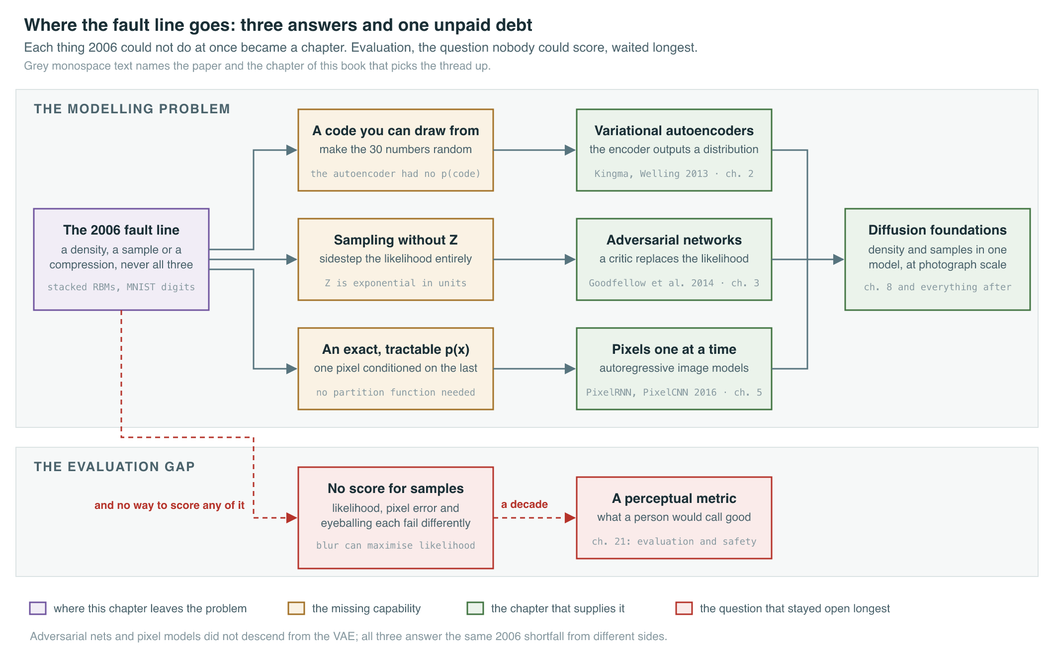
Neither 2006 paper produced anything that generated a convincing photograph, and neither was meant to. What they established was the vocabulary and the fault line the rest of this book’s first act runs along: a model can define a density, or support sampling, or compress well, and 2006 was the first time a single family of learned, multi-layer networks could be pointed at any one of those three jobs at will — just not, yet, at all three simultaneously for anything more complex than small grayscale digits and faces.

Capability	PCA / Gaussian mixture	RBM / deep belief net (2006)	Deep autoencoder (2006)	Where it gets resolved together
Defines an explicit density $p(x)$	yes, but poorly fits nonlinear manifolds	yes, via the energy function	no	Variational Autoencoders
Exact, tractable normalization	yes (closed form)	no — $Z$ is intractable beyond tiny networks	not applicable	Generative Adversarial Networks sidesteps likelihood entirely
Can sample a genuinely novel $x$	yes, but samples look blurred and generic	yes, by ancestral sampling downward	no — no distribution over its codes	Both chapters above, then Diffusion Foundations
Learns nonlinear latent structure	no	yes, via stacked hidden layers	yes, via the 30-dimensional bottleneck	Carried forward as “latent space” in every later chapter
Practical image scale, mid-2000s	small, low-resolution	small binary or grayscale images	small grayscale images	Natural photographs wait for the chapters above

The evaluation problem this era exposed turned out to be just as durable as the modeling problem. There was, in 2006, no agreed way to score how good a generative model’s samples looked to a person, and the two candidate proxies each failed differently.

Evaluation method	What it measures	Where it fails
Held-out log-likelihood	how much probability the model assigns to unseen real data	a model can maximize this while still producing blurry, low-quality samples; intractable to compute exactly for models like RBMs
Pixel reconstruction error	how closely an autoencoder’s output matches its input	rewards averaging over plausible details, producing blur, and says nothing about sampling from scratch
Human inspection	perceptual realism of generated samples	does not scale, is not reproducible across papers, and was the de facto standard throughout this era

That gap between a number a model can be trained against and a number that tracks what a human would call a good image persisted for another decade before a dedicated perceptual metric arrived — the subject of Evaluation, Provenance, and Safety.

Each thing 2006 could not do at once became a chapter of this book. Adversarial nets and pixel models did not descend from the VAE; all three answer the same shortfall from different sides, and evaluation waited longest. PNG ↓

Key Papers

Paper	Authors	Year	Link	Why it matters
Reducing the Dimensionality of Data with Neural Networks	Hinton and Salakhutdinov	2006	doi	Shows RBM-based layer-wise pretraining can initialize a deep autoencoder that beats PCA at compression — and shows, by omission, that a superb compressor is not automatically a generative model
A Fast Learning Algorithm for Deep Belief Nets	Hinton, Osindero, and Teh	2006	doi	Solves the depth problem for Boltzmann-style generative models, producing the first practical multi-layer network that both estimates a density and can be sampled top-down

PM Lens

The distinction this chapter draws between compressing and generating still shows up in the vendor demos I sit through today. A slick “AI image” pitch built entirely from cherry-picked prompts is, more often than I’d like, closer to Hinton and Salakhutdinov’s autoencoder than to a real generative system: it reconstructs things adjacent to what it has already seen and struggles the moment you ask for something with no near neighbor in its training data. The test I now run before trusting any such demo is close to the one this chapter’s math answers — can it sample something genuinely novel, or is it only ever interpolating? DALL-E 2’s public launch in April 2022 and Midjourney’s paid tiers, which started at $10 a month for its 2022 open beta, both had to survive exactly that kind of adversarial poking before I’d recommend either to a team. It took sixteen years to get from a 30-dimensional digit code to a system that could pass that test on open-ended prompts; the gap is worth remembering the next time a roadmap assumes it will close in one quarter.

Search