Keeping Training Alive

It is February 2015. Deep networks train, when they train at all, at the mercy of learning rates set an order of magnitude too conservative and initializations tuned by hand for every added layer. Two researchers at Google propose a fix that normalizes the activations flowing between layers, and within a year it is difficult to find a serious deep network that does not use some form of it. This chapter follows normalization from batches to layers to a single root-mean-square, and then follows a second, later thread — hyperparameters that transfer across model width — that keeps very large training runs from becoming unaffordable guesswork.

Where We Were

By the early 2010s, deep learning’s central practical obstacle was not a lack of ideas but the difficulty of actually training the networks those ideas required. Every layer’s weights update during training, which means every layer’s input distribution also shifts as training proceeds — the activations a layer receives at step 1,000 look statistically different from the activations it received at step 1. Each layer is effectively chasing a moving target, and the deeper the network, the more layers are chasing targets that are themselves moving because of the layers beneath them. The practical consequences were concrete: learning rates had to be kept small to avoid divergence, weight initialization had to be scaled with unusual care to keep activation variance from exploding or collapsing across depth, and saturating nonlinearities such as sigmoid and tanh were notoriously hard to train once a network had more than a handful of layers, because large pre-activations pushed them into flat regions with near-zero gradient.

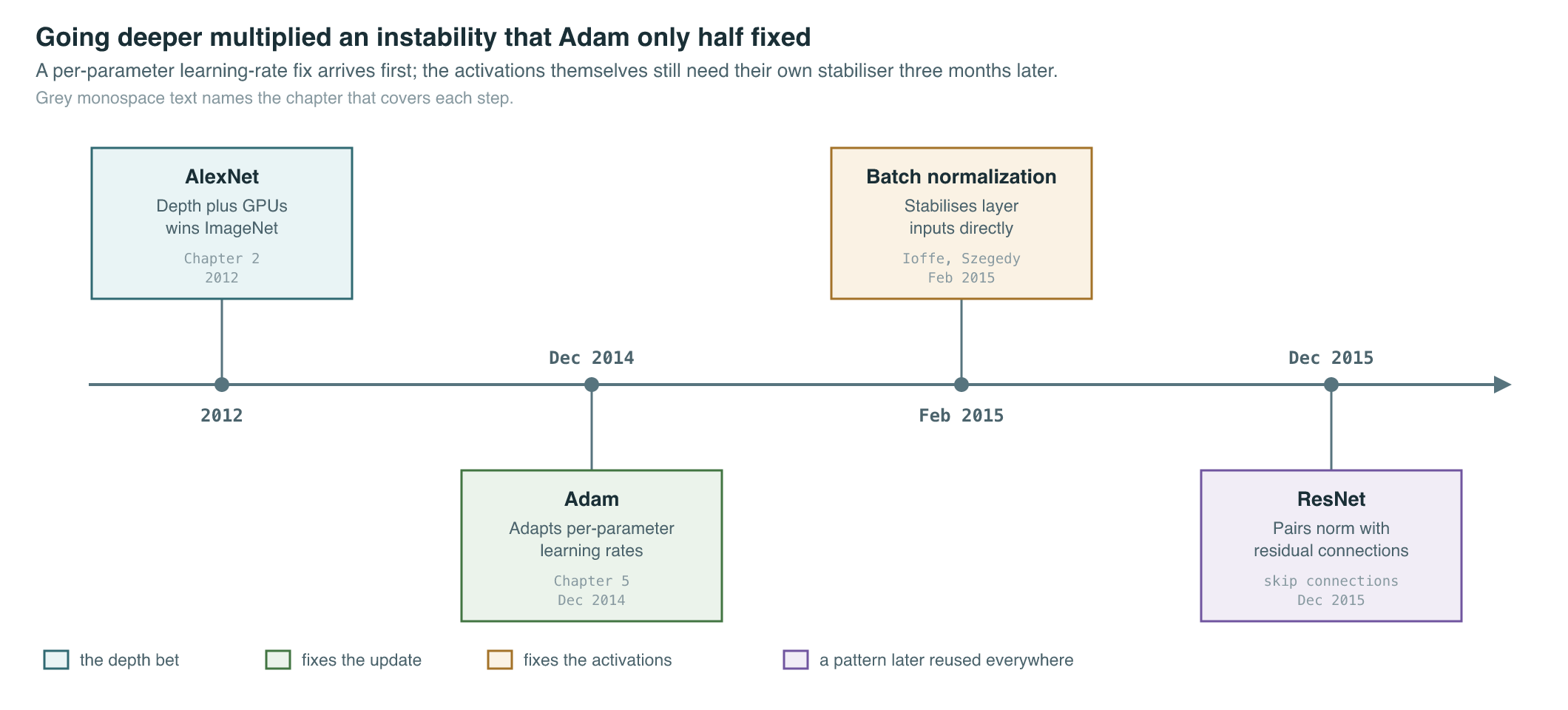
None of this was a niche concern. AlexNet’s 2012 breakout showed that depth plus GPU-scale compute could beat decades of hand-engineered computer vision, and the field’s obvious next move was to go deeper still. But going deeper multiplied exactly the instability described above. Adam (December 2014) — the per-parameter adaptive optimizer covered in Chapter 5 — helped by rescaling gradients per parameter, but it addressed the symptom of noisy, badly scaled gradients rather than the underlying drift in what each layer was seeing. Something had to stabilize the activations themselves, not just the updates computed from them.

Adam fixes the update three months before batch normalization fixes the activations themselves; going deeper needed both. PNG ↓

The Breakthrough

Batch normalization (Ioffe and Szegedy, 2015) reframed the problem: rather than asking the network to tolerate shifting input statistics, force those statistics to stay fixed. For each mini-batch during training, the method computes the mean and variance of each feature (each channel, each hidden unit) across the examples in the batch, subtracts the mean and divides by the standard deviation, and then applies a learned scale and shift so the layer can still represent whatever distribution is actually useful. The normalization is folded directly into the model architecture and differentiated through like any other operation, so the network learns around a fixed statistical baseline instead of a moving one.

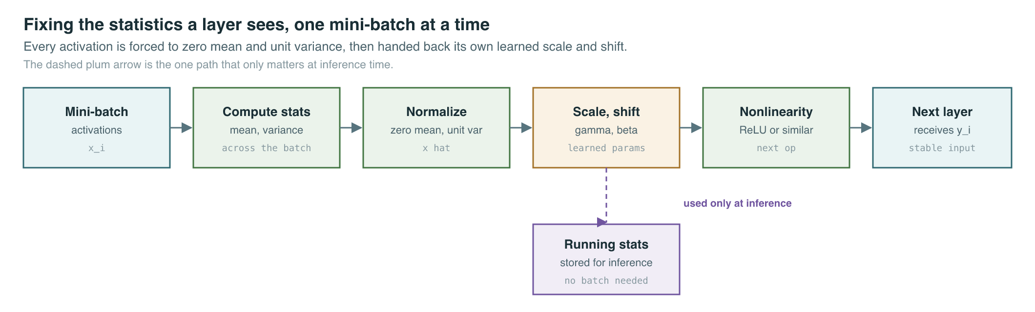
Everything left of the learned scale and shift happens the same way in training; only the dashed path, running statistics, exists purely to make inference work without a batch. PNG ↓

The paper’s own framing was internal covariate shift: by fixing the distribution each layer sees, the network no longer needs a small learning rate as insurance against distributional drift, and it no longer needs finely hand-tuned initialization to keep variance in a trainable range through depth. The reported effect on a state-of-the-art image classifier was large — the same accuracy in 14 times fewer training steps — and an ensemble of batch-normalized networks pushed the ImageNet top-5 error to 4.9% (4.8% on the test set), below the commonly cited human-rater error rate at the time. Batch normalization also turned out to act as an incidental regularizer: because each example’s normalization statistics depend on the other examples in its mini-batch, the network sees a slightly different transformation of the same input on every pass, an effect strong enough that some architectures dropped Dropout entirely.

The mechanism had a structural dependency, though: it normalizes across the batch dimension, which means it needs a batch of reasonable size to produce stable statistics, and at inference time — often on a single example — it has to fall back to running averages of mean and variance accumulated during training rather than statistics computed on the fly. That dependency was fine for the image classifiers of 2015, trained with batches in the hundreds. It was much less fine for recurrent networks processing variable-length sequences one step at a time, where “the batch” at a given timestep is a thin, awkward slice, and for any setting where per-device batches shrink — for instance under the large-scale data parallelism covered in Chapter 8, where splitting a batch across many accelerators can leave each device with only a handful of examples.

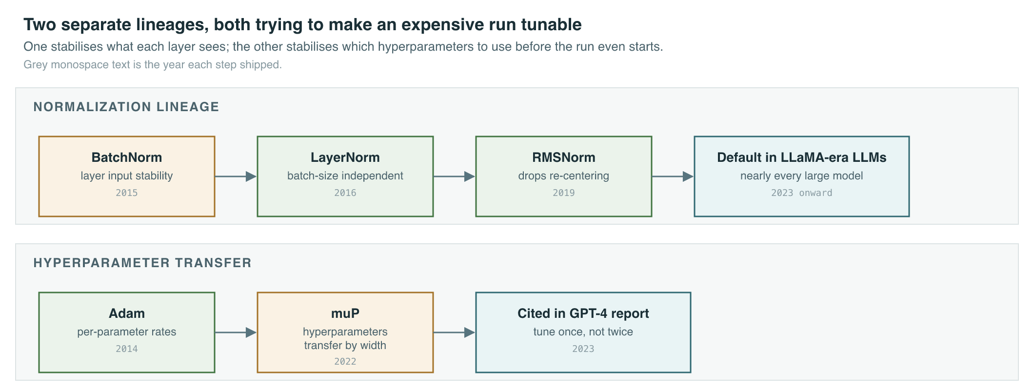
Layer normalization (Ba et al., 2016) removed the dependency by changing which dimension gets normalized. Instead of computing statistics across the examples in a batch, it computes them across the features of a single example — every example normalizes itself, using only its own activations. This makes the computation identical at training and inference time, indifferent to batch size, and a natural fit for recurrent networks and, later, the Transformer, whose sublayers are wrapped in exactly this normalization (full architecture in Language Models, Chapter 5).

Root mean square layer normalization (Zhang and Sennrich, 2019) asked a further question: does layer normalization need both of its two invariances? LayerNorm re-centers (subtracts the mean) and re-scales (divides by the standard deviation). RMSNorm’s authors hypothesized that the re-centering step was dispensable — that re-scaling alone, without computing and subtracting a mean, preserved the useful properties of normalization at a fraction of the compute, since dropping the mean removes an entire reduction and subtraction from every normalization call. Across a range of architectures and tasks, RMSNorm matched LayerNorm’s performance while cutting running time by 7% to 64%, and the simplification proved durable: it became the default normalization in most Transformer-based language models trained from the early 2020s onward, including LLaMA (February 2023) — covered in Language Models, Chapter 14.

Normalization solved instability within a fixed-size network. A separate instability problem appears the moment a team tries to scale that network up: hyperparameters tuned for one width rarely stay optimal at another, and for models with tens or hundreds of billions of parameters, running the equivalent of a grid search directly on the full-size model is not something most budgets tolerate. Tensor Programs V (Yang et al., 2022) introduced the maximal update parameterization (muP): a specific way of scaling initialization variance and learning rate with a network’s width such that a wide family of training dynamics stay stable and, crucially, such that the optimal hyperparameters stay the same across widths within that family. Tune a small proxy model cheaply, and the same hyperparameters transfer zero-shot to a much larger model in the same family — no retuning at scale required.

The Mathematics

Batch normalization’s core operation, applied per feature over a mini-batch, is:

\hat{x}_i = \frac{x_i - \mu_B}{\sqrt{\sigma_B^2 + \epsilon}}, \qquad y_i = \gamma\,\hat{x}_i + \beta

For each example $i$ in the mini-batch, $x_i$ is that feature’s raw activation, and $\mu_B$ and $\sigma_B^2$ are the mean and variance of this feature computed across every example currently in the batch $B$ . Subtracting the mean and dividing by the standard deviation (with a tiny $\epsilon$ added so nothing divides by zero) gives $\hat{x}_i$ , an activation forced to zero mean and unit variance regardless of what came before it in training. Because forcing every activation to exactly this shape would remove the network’s ability to represent anything else, a learned scale $\gamma$ and shift $\beta$ are applied afterward to recover whatever distribution the layer actually needs. What it buys you: the layer’s input statistics stop drifting as training proceeds, so you can raise the learning rate and relax initialization without the network diverging.

Symbol	Meaning
$x_i$	raw activation for example $i$ in the current feature
$\mu_B$	mean of this feature across the mini-batch $B$
$\sigma_B^2$	variance of this feature across the mini-batch $B$
$\epsilon$	small constant preventing division by zero
$\hat{x}_i$	normalized activation, zero mean and unit variance
$\gamma, \beta$	learned scale and shift, restoring representational freedom
$y_i$	the layer’s normalized output for example $i$

Layer normalization computes the same shape of transformation but along a different axis — across a single example’s own features, not across the batch:

\begin{aligned} \mu &= \frac{1}{d}\sum_{j=1}^{d} x_j, \qquad \sigma^2 = \frac{1}{d}\sum_{j=1}^{d} (x_j - \mu)^2 \\ y_i &= \gamma_i \cdot \frac{x_i - \mu}{\sqrt{\sigma^2 + \epsilon}} + \beta_i \end{aligned}

Symbol	Meaning
$d$	number of features in one example’s activation vector
$x_j$	the $j$ -th feature of the example being normalized
$\mu, \sigma^2$	mean and variance of that example’s own features
$x_i$	the specific feature being transformed
$\epsilon$	small constant preventing division by zero
$\gamma_i, \beta_i$	per-feature learned scale and shift
$y_i$	the normalized, rescaled output for feature $i$

RMSNorm drops the re-centering step entirely and normalizes only by the root mean square of the activations:

\mathrm{RMS}(x) = \sqrt{\frac{1}{d}\sum_{j=1}^{d} x_j^2 + \epsilon}, \qquad y_i = \gamma_i \cdot \frac{x_i}{\mathrm{RMS}(x)}

Symbol	Meaning
$d$	number of features in the example’s activation vector
$x_j$	the $j$ -th feature, used to compute the RMS statistic
$\epsilon$	small constant preventing division by zero
$x_i$	the specific feature being transformed
$\mathrm{RMS}(x)$	root-mean-square magnitude of the example’s features
$\gamma_i$	per-feature learned scale
$y_i$	the normalized, rescaled output for feature $i$

muP addresses a different variable entirely — not activation statistics within one network, but how hyperparameters should change as a network’s width changes. In its simplest form, for the hidden layers of a network family under muP, the learning rate and initialization variance at width $n$ are set relative to a tuned base width $n_0$ by:

\eta(n) = \eta_0 \cdot \frac{n_0}{n}, \qquad \sigma^2(n) = \sigma_0^2 \cdot \frac{n_0}{n}

Symbol	Meaning
$n_0$	width of the small, cheaply tuned proxy model
$n$	width of the full-size target model
$\eta_0, \eta(n)$	learning rate at the proxy width and at width $n$
$\sigma_0^2, \sigma^2(n)$	initialization variance at the proxy width and at width $n$

What It Enabled

Normalization did not stay confined to image classifiers. Within months, DCGAN (November 2015) — covered in Image Generation, Chapter 4 — leaned on batch normalization as one of its key stabilizers for what was, at the time, a famously unstable training procedure. Later that same year, ResNet paired normalization with residual connections (the skip-connection idea taught in Chapter 1) to push trainable depth past 100 layers; the two techniques became a standard combination, each addressing a different failure mode of very deep networks. As sequence models and then Transformers took over language modeling, LayerNorm’s independence from batch size made it the default, and RMSNorm’s efficiency gain made it the default’s default — a small, compounding saving multiplied across every layer of every forward and backward pass of every large model trained since.

	BatchNorm (2015)	LayerNorm (2016)	RMSNorm (2019)
Statistics computed over	features, across the batch	features, within one example	features, within one example
Depends on batch size	yes — needs running averages at inference	no	no
Re-centers (subtracts mean)	yes	yes	no
Best fit	fixed-size batches, image CNNs	sequences, variable batch size, Transformers	Transformers at scale
Reported efficiency claim	14x fewer steps to matched accuracy	—	7%–64% less running time than LayerNorm

muP’s effect was narrower but, at frontier scale, more consequential for project economics. Tensor Programs V reported that transferring hyperparameters tuned on a 13-million-parameter proxy surpassed published BERT-large (350M parameters) results at a tuning cost equivalent to a single BERT-large pretraining run, and that transferring from a 40-million-parameter proxy outperformed the released 6.7-billion-parameter GPT-3 model at only 7% of the typical pretraining compute for a model that size. OpenAI’s GPT-4 technical report states plainly that “it is not feasible to do extensive model-specific tuning” on a training run at that scale, and lists Tensor Programs V among its cited references — muP’s proxy-then-transfer method is one answer to the question every later chapter on frontier training runs has to confront: how do you tune something you can only afford to train once. Chapter 10 covers the companion question of how much compute a given model size and dataset size should receive; muP is the piece that lets you find good hyperparameters for that compute-optimal model without spending the same budget twice.

One lineage stabilises what a layer sees; the other stabilises which hyperparameters to use before an expensive run even starts. PNG ↓

Key Papers

Paper	Authors	Year	Link	Why it matters
Batch Normalization: Accelerating Deep Network Training by Reducing Internal Covariate Shift	Ioffe and Szegedy	2015	arXiv:1502.03167	First normalization layer folded into the architecture; let deep networks train with higher learning rates and looser initialization
Layer Normalization	Ba et al.	2016	arXiv:1607.06450	Removed the batch-size dependency by normalizing across features instead of across examples; became the Transformer’s default
Root Mean Square Layer Normalization	Zhang and Sennrich	2019	arXiv:1910.07467	Dropped re-centering to cut normalization cost by up to 64%; the default in most large language models trained after 2020
Tensor Programs V: Tuning Large Neural Networks via Zero-Shot Hyperparameter Transfer	Yang et al.	2022	arXiv:2203.03466	Introduced muP, letting hyperparameters tuned on a small proxy model transfer zero-shot to a much larger one

PM Lens

This is the chapter I point to whenever a training run I’m accountable for produces a loss curve with an unexplained spike. Normalization choices are usually invisible in a vendor’s marketing but visible immediately in a technical report’s appendix — LLaMA’s report says RMSNorm, in the same sentence as its architecture, because that sentence is load-bearing: get it wrong and the run doesn’t converge, full stop. The muP result is the more direct budget conversation. A team that can tune hyperparameters on a 40-million-parameter proxy and transfer them to a multi-billion-parameter run is not paying to discover, mid-training, that the learning rate was wrong — a failure mode that, at frontier scale, means restarting from a checkpoint and eating real GPU-hours. When I’m scoping a training-adjacent product bet, “how do you tune hyperparameters for a model you can only afford to train once” is now a standard diligence question, and “we don’t” is a real answer that changes my risk estimate.

Search