word2vec and the Geometry of Meaning

It is January 2013. Language models still treat words as unrelated symbols — “cat” and “kitten” are as distant as “cat” and “carburetor.” A short paper from a small team at Google shows that a stripped-down neural network, trained on billions of words in a day, arranges vocabulary in a vector space where meaning becomes geometry: king − man + woman lands next to queen.

Where We Were

The n-gram models of chapter 1 represented each word as an atomic symbol. In machine-learning terms, this is a one-hot vector: a vocabulary of $V$ words becomes a $V$-dimensional space in which each word occupies its own axis, orthogonal to every other word. The representation carries no notion of similarity — the model that has seen “the cat sat on the mat” learns nothing at all about “the kitten sat on the mat.” Every word must be learned from scratch, and the data requirements multiply accordingly.

Linguists had long suggested a way out. The distributional hypothesis — compressed by J.R. Firth in 1957 into “you shall know a word by the company it keeps” — holds that words appearing in similar contexts have similar meanings. By the 1990s and 2000s this idea had produced count-based methods such as latent semantic analysis, which factorized large word-document or word-word co-occurrence matrices into dense, low-dimensional vectors. These captured topical similarity reasonably well, but the vector spaces they produced had weak fine-grained structure, and building them meant handling enormous sparse matrices.

The neural route existed too. The neural probabilistic language model of Bengio et al. (2003), covered in chapter 1, learned a dense vector for each word as a byproduct of learning to predict the next word. The embeddings were real and useful — but the model around them was expensive. A hidden layer sat between the word vectors and the output, and the output itself was a softmax over the entire vocabulary. Training on more than a few hundred million words was impractical on the hardware of the era. Through 2012, word embeddings remained a niche curiosity: everyone agreed they were interesting, and almost nobody could afford to train good ones at scale.

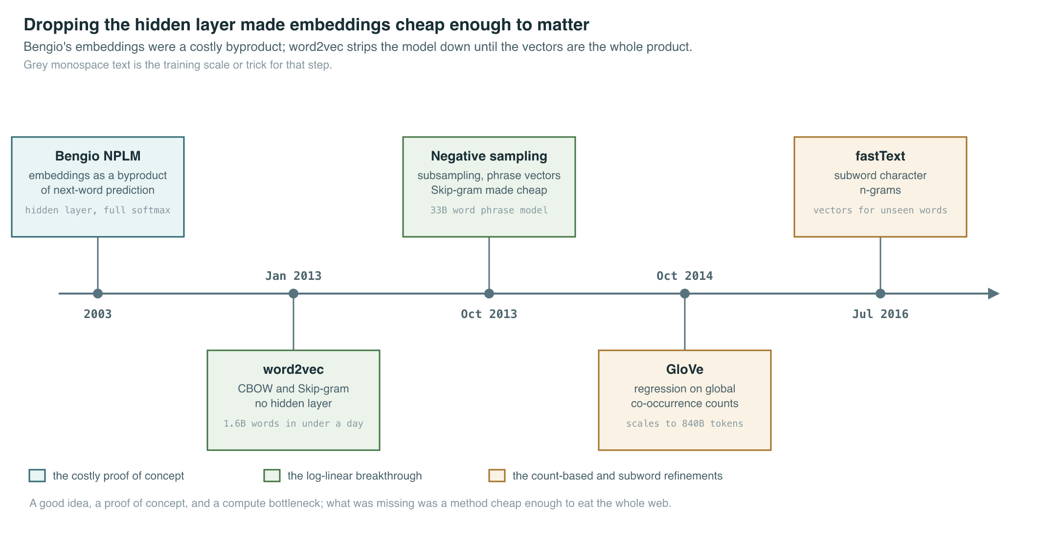
The stage, then: a good idea (dense vectors from context), a proof of concept (Bengio’s model), and a bottleneck (training cost). What was missing was a method cheap enough to eat the whole web.

The Breakthrough

word2vec (Mikolov et al., 2013) is less a new model than a strategic demolition. In “Efficient Estimation of Word Representations in Vector Space” (Mikolov et al., 2013), Tomas Mikolov, Kai Chen, Greg Corrado, and Jeffrey Dean asked what happens if you remove the expensive parts of the neural language model — the non-linear hidden layer above all — and keep only the embedding layer and a simple prediction task. The answer: quality goes up, because the compute you save buys you orders of magnitude more training data. The paper reports learning high-quality vectors from a 1.6-billion-word dataset in less than a day, and its main experiments use a Google News corpus of about 6 billion tokens with a vocabulary of one million words.

Two architectures share this design, differing only in the direction of prediction:

• CBOW (continuous bag-of-words) predicts the current word from an averaged window of surrounding words — four words of history and four of future in the paper’s configuration. Because the context vectors are averaged, word order inside the window is discarded, hence “bag of words.”
• Skip-gram inverts the task: given the current word, predict each word in a surrounding window (the paper samples context positions up to a maximum distance of $C = 10$). It is slower than CBOW but produced the strongest semantic vectors, and it is the variant the field adopted.

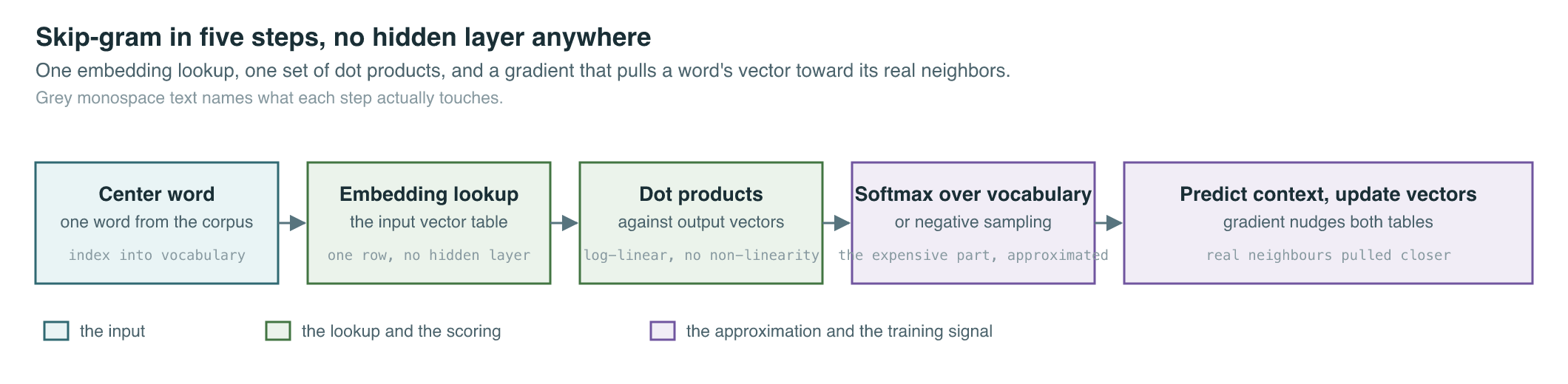
Both are log-linear models: one embedding lookup, one dot product per candidate word, no hidden layer. Each word gets two vectors — an input vector used when it is the center word and an output vector used when it is a context candidate — and training nudges the input vector of a word toward the output vectors of its actual neighbors.

The famous result is what this training produces as a side effect. The learned space supports vector arithmetic over meaning: the paper reports that vector(“King”) − vector(“Man”) + vector(“Woman”) is closest to the vector for Queen. To measure this systematically, the authors built a test set of 8,869 semantic and 10,675 syntactic analogy questions (“Athens is to Greece as Oslo is to ?”, “big is to bigger as cold is to ?”); their best Skip-gram configuration answered 66.1% of the semantic and 65.1% of the syntactic questions exactly — a striking figure given that an answer only counts if the nearest vector is precisely the right word. Directions in the space had become interpretable: one consistent offset encodes gender, another plurality, another country-capital relations.

Nine months later, “Distributed Representations of Words and Phrases and their Compositionality” (Mikolov et al., 2013) — the October 2013 follow-up with Ilya Sutskever joining the author list — made Skip-gram dramatically cheaper and better with three additions. Negative sampling replaced the full softmax with a handful of binary classifications (the mathematics below). Subsampling of frequent words randomly discarded a share of occurrences of very common words like “the” and “of,” which speeds training and, counterintuitively, improves the vectors of rare words by letting them see more informative contexts. And phrase vectors — treating “Air Canada” or “New York Times” as single tokens identified by a statistical pre-pass — extended the method beyond single words; trained on roughly 33 billion words, the phrase model reached 72% on a phrase-analogy test.

One year after that, GloVe (Pennington et al., 2014) arrived from Stanford as the count-based rejoinder (Pennington et al., 2014). Where Skip-gram streams through text window by window, GloVe first tallies a global word–word co-occurrence matrix, then fits vectors directly to the logarithms of those counts with a weighted least-squares regression. The result, in October 2014: a model that trains only on the nonzero cells of the matrix, reaches 75% on the same analogy task, and scales to corpora as large as 840 billion tokens of Common Crawl web data. Conceptually, GloVe demonstrated that the neural-prediction view (word2vec) and the matrix-factorization view (LSA’s descendants) were two roads to the same place — both distill co-occurrence statistics into geometry.

The Mathematics

Skip-gram maximizes the average log-probability of context words given center words. For a training corpus of $T$ words $w_1, \dots, w_T$:

$$\frac{1}{T} \sum_{t=1}^{T} \; \sum_{-c \le j \le c,\; j \ne 0} \log p\left(w_{t+j} \mid w_t\right)$$

Symbol	Meaning
$T$	number of words in the training corpus
$w_t$	the center word at position $t$
$w_{t+j}$	a context word $j$ positions away
$c$	context window radius
$p(w_{t+j} \mid w_t)$	model probability of seeing that context word

The probability itself is defined by a softmax over dot products of the two vector tables:

$$p\left(w_O \mid w_I\right) = \frac{\exp\left({v'}_{w_O}^{\top} v_{w_I}\right)}{\sum_{w=1}^{V} \exp\left({v'}_{w}^{\top} v_{w_I}\right)}$$

Symbol	Meaning
$w_I, w_O$	input (center) word and output (context) word
$v_w$	input vector of word $w$
$v'_w$	output vector of word $w$
$V$	vocabulary size

The first paper escaped the denominator with a hierarchical softmax (a binary tree over the vocabulary, cost $\log_2 V$ instead of $V$). The October paper introduced the simpler and now-canonical escape, negative sampling, which replaces each softmax term with:

$$\log \sigma\left({v'}_{w_O}^{\top} v_{w_I}\right) + \sum_{i=1}^{k} \mathbb{E}_{w_i \sim P_n(w)}\left[\log \sigma\left(-{v'}_{w_i}^{\top} v_{w_I}\right)\right]$$

Symbol	Meaning
$\sigma(x)$	logistic sigmoid, $1/(1+e^{-x})$
$k$	number of negative samples per real pair
$P_n(w)$	noise distribution, $\propto U(w)^{3/4}$ where $U$ is the unigram frequency
$\mathbb{E}$	expectation — in practice, average over the $k$ sampled words

The same paper’s subsampling trick discards each occurrence of word $w_i$ with probability:

$$P\left(w_i\right) = 1 - \sqrt{\frac{t}{f\left(w_i\right)}}$$

GloVe reaches similar geometry from the opposite direction. Let $X_{ij}$ count how often word $j$ appears in the context of word $i$ across the whole corpus. GloVe minimizes:

$$J = \sum_{i,j=1}^{V} f\left(X_{ij}\right) \left( w_i^{\top} \tilde{w}_j + b_i + \tilde{b}_j - \log X_{ij} \right)^2$$

Symbol	Meaning
$X_{ij}$	global co-occurrence count of words $i$ and $j$
$w_i, \tilde{w}_j$	word vector and context vector being learned
$b_i, \tilde{b}_j$	scalar bias terms
$f(\cdot)$	weighting function capping frequent pairs
$V$	vocabulary size

The deeper unity: Skip-gram sees local windows one at a time; GloVe sees all windows at once, pre-aggregated into counts. Both end up encoding the same co-occurrence statistics, which is why their vector spaces behave so similarly.

What It Enabled

The immediate effect was a representation upgrade for the entire field. Between 2013 and 2018, virtually every neural NLP system began with a pretrained embedding table — often the released Google News word2vec vectors or Stanford’s downloadable GloVe vectors (trained on corpora from a 6-billion-token Wikipedia + Gigaword mix up to 840 billion tokens of Common Crawl, at 50 to 300 dimensions).

	One-hot / n-gram (before)	Dense embeddings (after)
Dimensions per word	$V$ (≈ 10⁵–10⁶), all but one zero	50–1,000, all informative
”cat” vs “kitten”	orthogonal — zero similarity	nearby vectors
Word relations	not representable	vector offsets (gender, tense, capital-of)
Unseen contexts	must be observed verbatim	generalize via neighborhood
Transfer across tasks	none	pretrain once, reuse everywhere
Training cost	counting	under a day for 1.6B words on CPUs, 2013

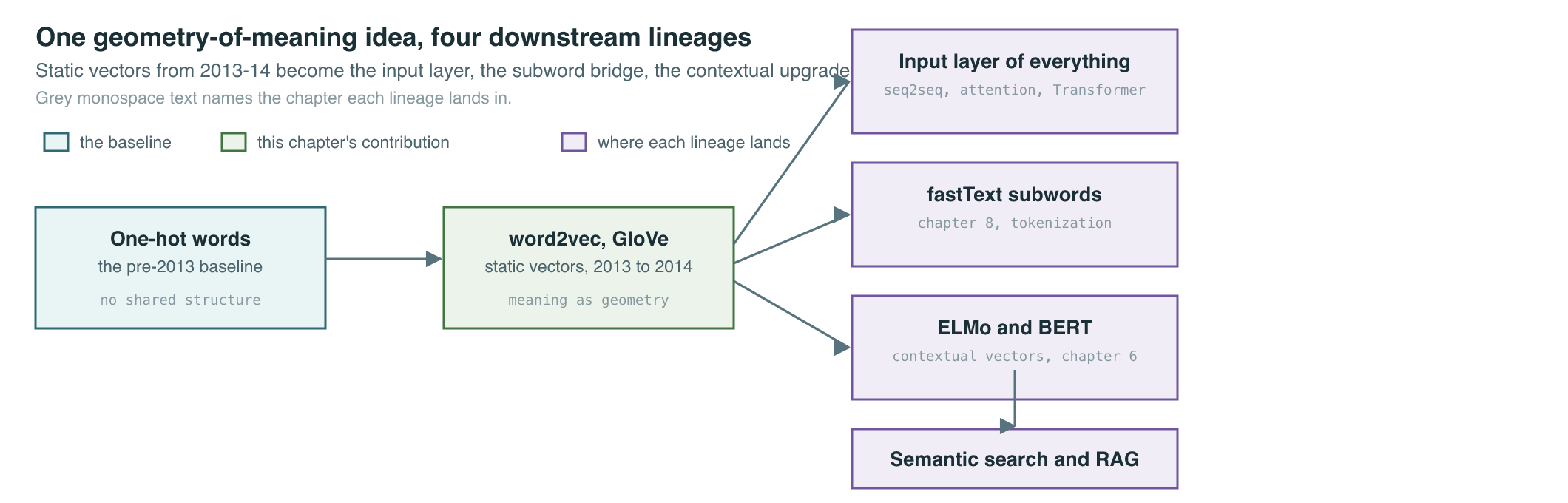
Three lineages flow directly out of this chapter:

Embeddings became the input layer of everything. The sequence-to-sequence models of chapter 3 consume word vectors, the attention mechanism of chapter 4 computes dot products between them, and the Transformer of chapter 5 is, at one level of description, a machine for repeatedly refining token embeddings. The “embedding table + gradient descent” pattern word2vec popularized is still the first layer of every modern LLM.

Static vectors exposed their own ceiling. A single vector per word type means bank (river) and bank (finance) share one point in space — polysemy is averaged away. fastText (Bojanowski et al., 2016) patched a different weakness, representing words as bags of character n-grams so that morphology is shared and out-of-vocabulary words get vectors (Bojanowski et al., 2016) — a step on the road to the subword tokenizers of chapter 8. But the polysemy problem demanded contextual embeddings — a different vector for each occurrence, computed by a full language model. ELMo and BERT delivered exactly that in 2018, and chapter 6 tells that story.

Semantic search was born here. The idea that meaning-similarity equals vector-proximity — nearest-neighbor lookup in embedding space — is the conceptual core of today’s retrieval-augmented systems and vector databases, covered in chapter 17. What changed between 2013 and now is what gets embedded (sentences and documents rather than word types) and by what (Transformers rather than log-linear models); the geometry-of-meaning premise is unchanged.

	word2vec Skip-gram	GloVe	fastText
Year	2013	2014	2016
Signal	local context windows, streamed	global co-occurrence matrix	local windows + character n-grams
Training	negative-sampling SGD	weighted least squares on nonzero counts	negative-sampling SGD
Unknown words	no vector	no vector	composed from subwords
Notable scale	~33B words (phrase model)	up to 840B tokens	multilingual releases

A closing caution on what the analogies did and did not show. The parallelogram demo was a brilliant evaluation — it made vector quality visible to anyone in one line — but it also revealed that embeddings inherit whatever statistical regularities the corpus contains, including social stereotypes encoded in co-occurrence patterns. That observation seeded the embedding-bias literature and, later, entire evaluation and alignment agendas (chapter 22).

Key Papers

Paper	Authors	Year	Link	Why it matters
Efficient Estimation of Word Representations in Vector Space	Mikolov et al.	2013	arXiv:1301.3781	CBOW and Skip-gram; deleted the hidden layer, traded model capacity for data scale; the analogy test
Distributed Representations of Words and Phrases and their Compositionality	Mikolov et al.	2013	arXiv:1310.4546	Negative sampling, frequent-word subsampling, phrase vectors — made Skip-gram the field’s default
GloVe: Global Vectors for Word Representation	Pennington et al.	2014	ACL Anthology	Regression on global co-occurrence counts; unified the count-based and prediction-based views
Enriching Word Vectors with Subword Information	Bojanowski et al.	2016	arXiv:1607.04606	Character n-gram composition; vectors for rare and unseen words; the bridge toward subword tokenization

PM Lens