Why Video Is Hard

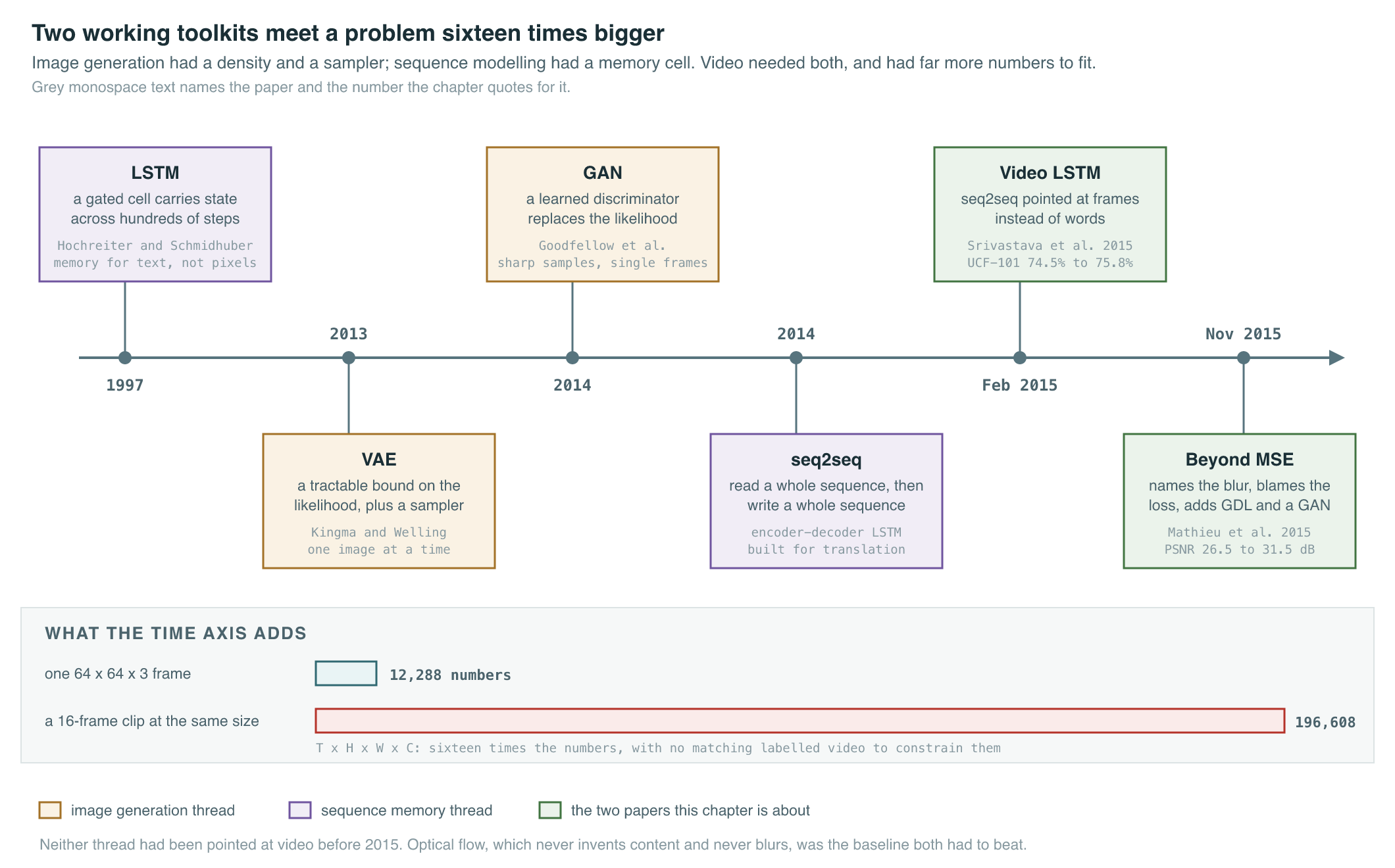
It is February 2015. Image generation already has a working, if imperfect, vocabulary — a density and a sampler, competing over how to get both from the same network — and sequence models already have a working memory cell for text that spans hundreds of steps. Neither thread has been pointed at video, where a “sample” is not one image but many, arranged in an order that itself carries most of the meaning. Within nine months, two papers establish the same unwelcome fact from two different angles: taught the straightforward way, a network that predicts what a video does next settles for a blur, and getting past that blur means changing what the network is asked to minimize, not just how big it is.

Where We Were

By early 2015 the generative-modeling toolkit for single images had two working answers to the two-job problem of density estimation and sampling: the variational autoencoder (VAE), which optimizes a tractable bound on log-likelihood, and the generative adversarial network (GAN), which sidesteps likelihood with a learned discriminator — both covered in full in the image-generation book, which also covers the GAN objective. Sequence modeling for text had its own working answer to a different problem — not “generate a plausible instance” but “carry information across an arbitrary number of steps” — solved by the long short-term memory (LSTM) cell and refined into an encoder-decoder pattern that reads a whole input sequence before generating a whole output sequence, the subject of Recurrent Networks and seq2seq.

Video sits at the intersection and inherits the hard parts of both problems without inheriting a ready-made combined solution. A single video frame is already the same high-dimensional object an image model has to handle — height times width times color channels, tens of thousands of numbers for even a modest resolution. A video multiplies that by however many frames the clip contains, and does so without a matching increase in the labeled data available to constrain the extra dimensions: ImageNet-scale labeled still-image datasets existed by 2015, but nothing comparable existed for labeled video motion. Worse, the added axis is not just “more of the same kind of number” — frames are not independent samples the way images in a dataset are; frame $t+1$ is heavily constrained by frame $t$ , in ways a model has to discover (objects persist, motion is usually smooth, occlusion and revealment happen at object boundaries) rather than being told.

There was also, in 2015, a strong non-learned baseline sitting in the way of any new video model’s claim to progress: optical flow. Decades of computer vision research had produced algorithms that estimate, for each pixel, how it moved between two frames, without training a generative model at all — a mature, well-understood technique for a narrower task than full frame prediction. Any learned video model claiming an advance had to beat not only the previous learned model, but a classical method with no training data requirement and no blur problem, because it never predicts new content — it only rearranges pixels that were already there.

Two mature toolkits, neither yet pointed at video, and the reason video needed more than either: a clip carries sixteen times the numbers of a frame without sixteen times the labels to pin them down. PNG ↓

The Breakthrough

The breakthrough arrived in two acts, nine months apart, attacking two different halves of the same underlying problem: the first act asks what a network should learn from unlabeled video at all; the second asks why, once it learns something, its predictions look wrong.

Act one: treat a video like a sentence. Srivastava, Mansimov, and Salakhutdinov (February 2015) applied the encoder-decoder LSTM framework, already established for translation, directly to raw video (Srivastava, Mansimov & Salakhutdinov, 2015). Where seq2seq feeds one word per time step into an encoder LSTM and decodes one word per time step out of a second LSTM, this paper feeds one video frame per time step — either a raw $32 \times 32$ pixel patch or a 4096-dimensional “percept” vector extracted from an ImageNet-pretrained convolutional network — and asks a decoder LSTM to produce a target sequence of frames. The paper tests three decoder targets. An Autoencoder Model decodes the same frames it was given, in reverse order, forcing the fixed-length encoder state to retain enough to reconstruct the input — a video-specific version of the deterministic compression problem covered for images in The Generative Problem. A Future Predictor Model decodes the frames that come after the input sequence instead, forcing the encoder state to capture motion well enough to extrapolate it. A Composite Model runs both decoders off one shared encoder, so the learned representation has to support reconstruction and extrapolation simultaneously — which the paper argues prevents each individual failure mode: a pure autoencoder can cheat by memorizing enough to reconstruct without learning anything about motion, and a pure future predictor can cheat by attending only to the last few input frames rather than the whole sequence.

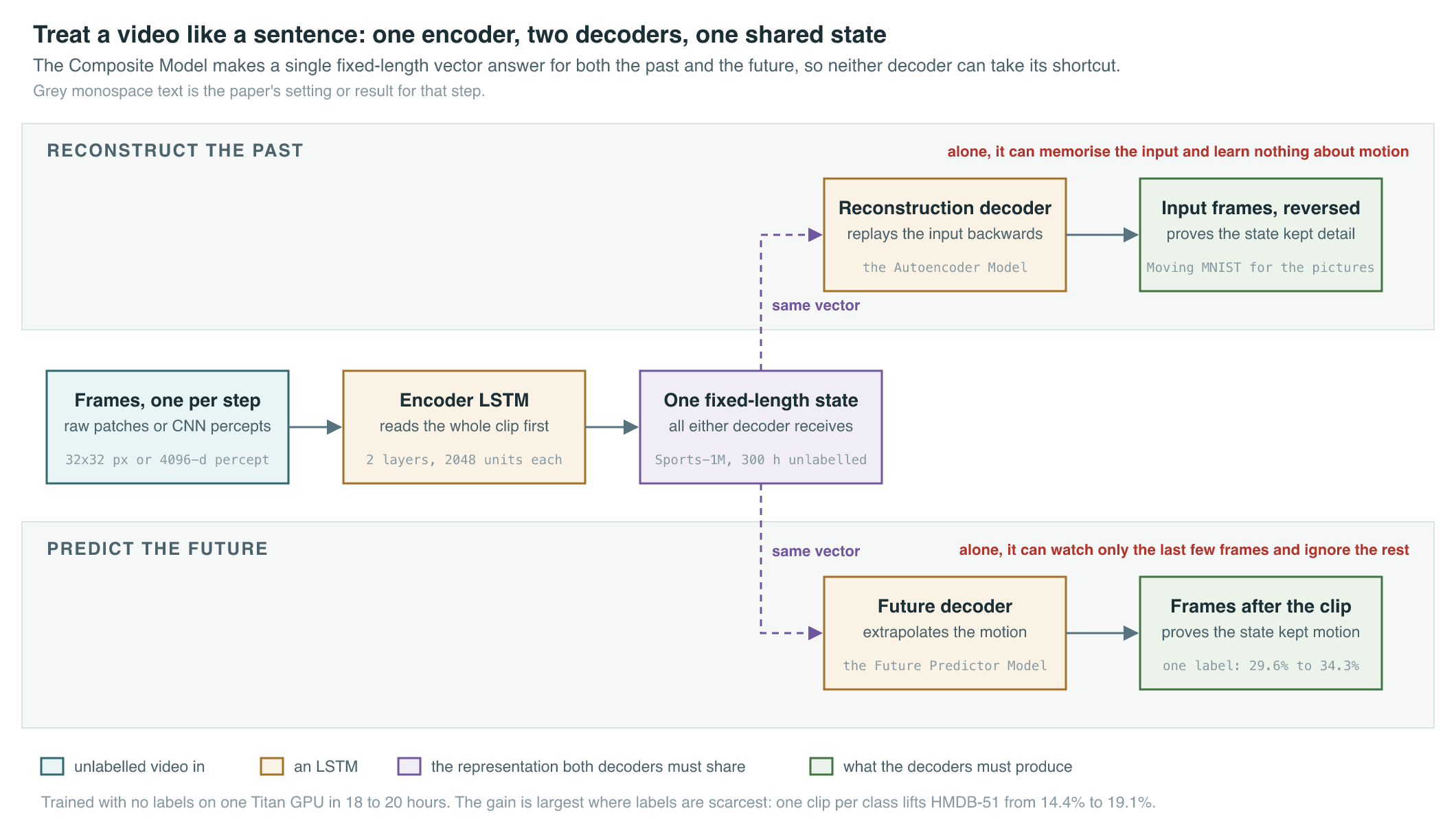
The Composite Model's trick is the single shared vector: it has to hold enough detail to rebuild the past and enough motion to extend the future, so neither decoder's shortcut survives. PNG ↓

Trained on a 300-hour subset of unlabeled YouTube clips from the Sports-1M dataset, plus a synthetic Moving MNIST dataset of digits bouncing inside a frame for controlled visualization, the best Composite Model used two stacked layers of 2048 or 4096 LSTM units. The result the paper is built around: features learned with no labels at all, by nothing more than reconstructing the past and predicting the future, transfer to a supervised action-recognition task, and the transfer benefit is largest exactly where labeled examples are scarcest. On the full UCF-101 dataset, fine-tuning from Composite Model weights raised classification accuracy from a 74.5% LSTM baseline to 75.8%; on HMDB-51, from 42.8% to 44.1%. With only one labeled video per class, the gap widened sharply — UCF-101 accuracy rose from 29.6% to 34.3%, HMDB-51 from 14.4% to 19.1%.

Act two: diagnose the blur, then fix the loss. Mathieu, Couprie, and LeCun (November 2015) started from a different question: given a network trained to predict the next frame directly in pixel space, why do its outputs look soft and smeared rather than sharp, no matter how the architecture is tuned (Mathieu, Couprie & LeCun, 2015)? Their answer, worked out in full in the next section, is that the standard squared-error (MSE, or $\ell_2$ ) loss used almost everywhere else in supervised deep learning is mathematically the wrong tool whenever a video’s future is genuinely uncertain. The paper proposes three complementary fixes, trained together on one convolutional generator. A multi-scale architecture predicts recursively from coarse resolution upward — four scales in their main experiments, from $4 \times 4$ patches up to $32 \times 32$ , later fine-tuned at $64 \times 64$ — each scale predicting a correction added to an upsampled coarser prediction, addressing the limited receptive field of a single-scale convolutional network. Adversarial training adapts the GAN, covered for images in The Adversarial Game, to frame prediction for the first time: a discriminator network looks at a full sequence of frames and predicts whether its last frames are real continuations or network-generated ones, which lets it exploit temporal coherence across the whole clip rather than judging one frame in isolation. And a new Gradient Difference Loss (GDL), described with its exact formula in the next section, directly penalizes mismatches between the predicted frame’s spatial edges and the true frame’s spatial edges, independent of whether raw pixel intensities line up.

A pixel loss stays as the backbone; the edge loss and the discriminator are bolted on to stop the generator averaging its futures. The bars show what that bought, and how narrowly it edged past optical flow. PNG ↓

The Mathematics

How much bigger video is than an image. The dimensionality gap between the two problems this book is about is not subtle:

D_{\text{image}} = H \times W \times C, \qquad D_{\text{video}} = T \times H \times W \times C

An image’s dimensionality is its height $H$ times its width $W$ times its number of color channels $C$ — around 12,288 numbers for a modest $64 \times 64 \times 3$ frame. A video clip’s dimensionality multiplies that by the number of frames $T$ : a 16-frame clip at the same resolution is 196,608 numbers, sixteen times larger, for content that is visually almost the same amount of “stuff.” This buys nothing on its own — it is the size of the problem, not a solution to it — but it is the reason every architectural choice in this chapter’s two papers (patch-based training, multi-scale prediction, compressed “percept” inputs instead of raw pixels) exists: full-resolution, many-frame video did not fit in 2015 GPU memory or training time without some form of dimensionality reduction first.

Symbol	Meaning
$H, W$	frame height and width, in pixels
$C$	number of color channels
$T$	number of frames in the clip
$D_{\text{image}}, D_{\text{video}}$	total dimensionality of one image versus one clip

Why squared-error prediction blurs. Mathieu et al. trace the blur to a basic fact about what squared error minimizes. For a scalar target $v$ drawn from some distribution, the value that minimizes expected squared error against it is the distribution’s mean, not any value the distribution is likely to actually produce:

\hat v^{*} = \arg\min_{\hat v} \; \mathbb{E}\big[(v - \hat v)^2\big] = \mathbb{E}[v]

$\mathbb{E}[v]$ is the expected value — the probability-weighted average — of the target $v$ . This equation says the single best guess $\hat v^{*}$ under squared-error loss is always that average, regardless of what the underlying distribution of $v$ actually looks like. If a pixel’s true next value could plausibly be either of two very different values $v_1$ or $v_2$ with roughly equal probability — a ball’s edge that could move left or right — the loss-minimizing prediction is their midpoint, $v_{\text{avg}} = (v_1 + v_2)/2$ , even though that midpoint value never occurs in any real frame and looks like neither outcome. This is not a training failure to be fixed with more data or a bigger network: it is what the loss function is defined to produce whenever the future is genuinely multi-modal, which video almost always is. It is the single equation this chapter’s subtitle — the blurry-MSE lesson — is named for, and it recurs, in different guises, every time a later chapter’s model reaches for a plain regression loss against pixels.

Symbol	Meaning
$v$	the true (uncertain) target value, e.g. one pixel’s next-frame intensity
$\hat v$	a candidate prediction
$\hat v^{*}$	the squared-error-optimal prediction
$\mathbb{E}[\cdot]$	expectation — the probability-weighted average
$v_1, v_2, v_{\text{avg}}$	two equally likely outcomes and their midpoint

The fix: penalize blurred edges directly. The Gradient Difference Loss compares spatial gradients — simple pixel-to-neighbor differences — of the predicted frame $\hat Y$ against the ground-truth frame $Y$ , rather than comparing raw pixel values:

\mathcal{L}_{gdl}(Y, \hat Y) = \sum_{i,j} \Big( \big| \,|Y_{i,j} - Y_{i-1,j}| - |\hat Y_{i,j} - \hat Y_{i-1,j}|\, \big|^{\alpha} + \big| \,|Y_{i,j-1} - Y_{i,j}| - |\hat Y_{i,j-1} - \hat Y_{i,j}|\, \big|^{\alpha} \Big)

For every pixel location $(i, j)$ , the terms $|Y_{i,j} - Y_{i-1,j}|$ and $|Y_{i,j-1} - Y_{i,j}|$ are finite-difference approximations of the true frame’s edge strength in the vertical and horizontal directions; the corresponding $\hat Y$ terms are the same measurement on the prediction. The loss is the total mismatch between these two edge maps, raised to a power $\alpha \geq 1$ that controls how sharply large mismatches are penalized. What this buys: a network can satisfy this loss only by reproducing the true frame’s edges at full strength, which is exactly the property the argument above shows plain squared error destroys — an average of two shifted edges is a soft, low-contrast edge, and GDL penalizes that softness directly rather than hoping a pixel-value loss will produce sharpness as a side effect. GDL is added to, not substituted for, an $\ell_p$ pixel loss and the adversarial loss below; the three are complementary fixes for three different symptoms of the same underlying problem.

Symbol	Meaning
$Y, \hat Y$	ground-truth and predicted frame
$i, j$	pixel row and column indices
$\alpha$	integer exponent, $\geq 1$ , controlling penalty sharpness
$\mathcal{L}_{gdl}$	the total gradient-difference loss over the frame

Combining the three losses. The generator $G$ is trained to minimize a single weighted sum:

\mathcal{L}(X, Y) = \lambda_{adv}\, \mathcal{L}^{G}_{adv}(X, Y) + \lambda_{\ell_p}\, \mathcal{L}_p(X, Y) + \lambda_{gdl}\, \mathcal{L}_{gdl}(X, Y)

Three loss terms are added together with hand-set weights $\lambda_{adv}$ , $\lambda_{\ell_p}$ , and $\lambda_{gdl}$ : an adversarial term $\mathcal{L}^{G}_{adv}$ (the video-specific adaptation of the GAN objective taught in The Adversarial Game), a standard $\ell_p$ pixel-distance term $\mathcal{L}_p$ , and the gradient-difference term above. In the paper’s best-performing configuration the weights were $\lambda_{adv} = 0.05$ , $\lambda_{\ell_p} = 1$ , and $\lambda_{gdl} = 1$ — the adversarial term contributes a small correction on top of a pixel-loss backbone rather than dominating training, because an adversarial loss used alone is prone to instability (the generator can learn to “confuse” a fixed discriminator without actually getting closer to the ground truth). This recipe — a stable regression loss as the backbone, with one or more additional terms bolted on to fix a specific known failure mode — recurs throughout the generative-modeling literature that follows, including well outside video.

Symbol	Meaning
$X, Y$	input frames and the ground-truth target frame
$\mathcal{L}(X, Y)$	the total training loss for the generator
$\mathcal{L}^{G}_{adv}(X, Y)$	the adversarial term, from the discriminator’s judgment of the generator’s output
$\mathcal{L}_p(X, Y)$	the standard $\ell_p$ pixel-distance term
$\mathcal{L}_{gdl}(X, Y)$	the gradient-difference term defined above
$\lambda_{adv}, \lambda_{\ell_p}, \lambda_{gdl}$	hand-set weights on the three terms

What It Enabled

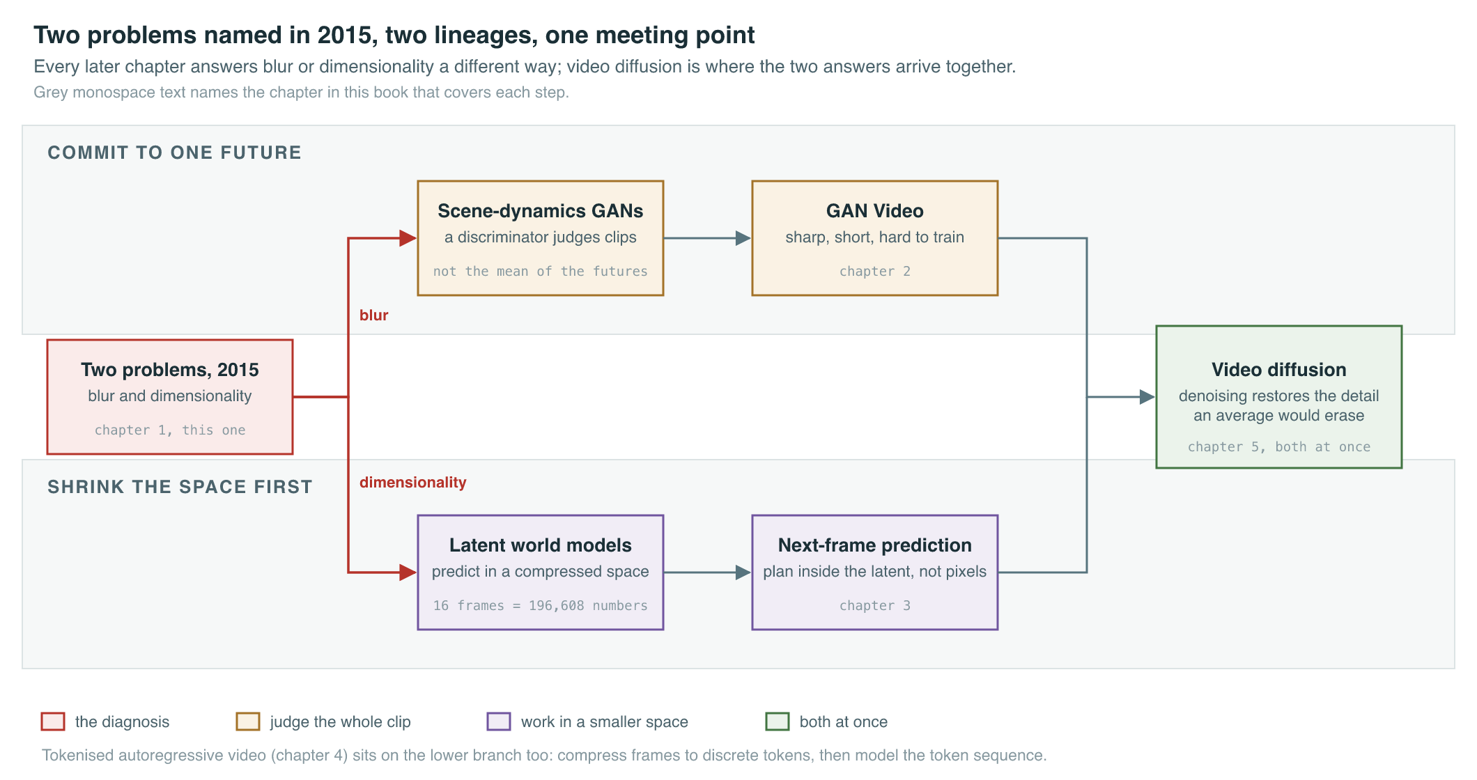
Neither 2015 paper produced a video model anyone would call visually convincing by later standards, and neither claimed to. What they established were the two problems every later chapter in this book answers a different way: how to represent a clip’s dimensionality without training on raw, full-length pixel tensors, and how to keep a learned predictor from collapsing to the statistically safe average of an uncertain future.

Approach	How it handles the time axis	How it handles (or falls into) blur	Where it’s covered
Classical optical flow, pre-2015	Estimates per-pixel motion between two real frames; generates nothing new	Sharp by construction — it only moves existing pixels — but cannot invent occluded or novel content	Baseline throughout this era
Video LSTM Composite Model, Feb 2015	Learns a fixed-length latent state via an encoder-decoder LSTM, decoded into a future sequence	Trained with plain squared or cross-entropy error; reconstructions and predictions are visibly blurry	This chapter
Multi-scale adversarial predictor, Nov 2015	Feed-forward convolutional network, no recurrence; predicts one or a few frames at a time	Loss function engineered against blur directly (GDL plus adversarial term); still limited to a short prediction horizon	This chapter
GAN-based video generation	A discriminator judges a full generated clip’s realism rather than scoring per-pixel accuracy	GAN Video
Latent world models	Predicts and plans inside a learned, compressed latent space instead of pixel space	Predicting the Next Frame
Tokenized autoregressive video	Compresses frames to discrete tokens first, then models the token sequence	Tokens for Video
Video diffusion models	Iterative denoising sampling reintroduces stochastic detail an average would erase	Video Diffusion Models

The 2015 quantitative record itself is worth keeping, because it shows how close the gap to a decades-old, non-learned baseline still was. Mathieu et al.’s evaluation on UCF-101, restricted to moving image regions and predicting one frame from four inputs, measured Peak Signal-to-Noise Ratio (PSNR), Structural Similarity (SSIM), and a purpose-built sharpness-difference score:

Loss configuration	PSNR (dB)	SSIM	Sharpness (dB)
Single-scale squared error	26.5	0.84	24.7
Absolute-error loss	28.7	0.88	24.8
Gradient difference loss + absolute error	29.4	0.90	25.0
Adversarial loss alone	30.6	0.89	25.2
Adversarial + gradient difference loss	31.5	0.91	25.4
Adversarial + gradient difference, fine-tuned on UCF-101	32.0	0.92	25.4
Non-learned optical-flow baseline	31.6	0.93	25.3

Every engineered fix improved on plain squared error, and the best combination edged past the classical optical-flow baseline on two of three measures — but only barely, and only after specifically fine-tuning on the test domain. Sharper video generation, in other words, did not arrive by scaling a squared-error model; it arrived by first proving that squared error was structurally the wrong objective, a lesson GAN Video and every later chapter’s model absorbs in its own way.

Every later chapter picks up one of the two problems this one names. Video diffusion is where the two lineages arrive together: a compressed space to work in, and a sampler that puts back the detail an average would erase. PNG ↓

Key Papers

Paper	Authors	Year	Link	Why it matters
Unsupervised Learning of Video Representations using LSTMs	Srivastava, Mansimov & Salakhutdinov	2015	arXiv	First encoder-decoder LSTM applied directly to video frames; shows unsupervised pretraining helps action recognition most exactly when labeled data is scarcest
Deep Multi-Scale Video Prediction Beyond Mean Square Error	Mathieu, Couprie & LeCun	2015	arXiv	Proves why squared-error frame prediction blurs, and fixes it with a multi-scale architecture, the first video GAN, and a new gradient-difference loss

PM Lens

The failure mode this chapter names — a network trained to minimize squared pixel error settles for the average of several plausible futures rather than committing to one — is still the first thing I check when a vendor demos a video model. Confident, wrong-in-one-direction output is usually a better product experience than the double-exposure blur Mathieu, Couprie, and LeCun measured back in November 2015, even though blur is technically the “safer” number on a squared-error scoreboard. Every commercially shipped text-to-video product since has solved this the same structural way these two 2015 papers first proved out — Stable Video Diffusion’s open-weight release in November 2023, Runway’s Gen-3 Alpha in mid-2024, Google’s Veo line announced that same May — by swapping or augmenting a plain regression loss with something that judges a whole sequence’s plausibility, not its per-pixel closeness to one ground truth. A roadmap that proposes “just add more training data” to fix blurry or flickery video output is treating a loss-function problem as a data problem, and it will not converge.

Search